• Premier League Historical Statistics

    Interactive Visualization of 15 years of England’s Football Premier League – a non-competitive Contribution to Tableau’s “Interactive Sports Viz Contest”

    Premier League LogoLast week, Tableau announced a new visualization contest: The Tableau Interactive Sports “Viz” Contest.

    Intrigued with the very attractive prices Tableau announced, I would have loved to contribute a workbook. Unfortunately, I am not allowed to, because the contest is open to US residents only.

    If you are a regular reader of this blog, you may have noticed that I love using sports data for my examples. We had several visualizations (Tableau and/or Excel) of Football statistics and even one article using Baseball data:

    Since I am so into visualizing sports data, I decided to publish the workbook I would have contributed to the contest: a Tableau visualization of 15 years of historical data of the English Premier League.

    Today’s article provides the workbook for direct interaction here or for download from Tableau Public. A follow-up post later this week will describe step-by-step tutorials of some of the most interesting techniques I used for the implementation.
    (more…)

  • Emulate Excel Pivot Tables with Texts in the Value Area using VBA

    How to create a Microsoft Excel Pivot Table lookalike Crosstab with Texts in the Value Area using VBA

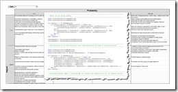
    Pivot Tables with Texts (VBA version) - click to enlargeThe recent post showed a way how to create a Pivot Table lookalike crosstab with texts in the value area.

    However, due to the fact that it was restricted to Excel formulas, the approach came with a couple of drawbacks. Using formulas forces you to define the layout and the size of the crosstab in advance in a static structure. It goes without saying that this considerably limits the usability in real life.

    Without VBA, there is no way out. However, some VBA helps to overcome almost all of the disadvantages of the formula based approach. Today’s post is the announced follow-up: it describes how to use VBA to emulate a Pivot Table lookalike crosstab with texts in the value area, as always including the Excel workbook for free download.

    (more…)

  • Emulate Excel Pivot Tables with Texts in the Value Area using Formulas

    How to create a Microsoft Excel Pivot Table lookalike Crosstab with Texts in the Value Area using Array Formulas

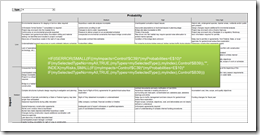
    Pivot Tables with Texts (Formula Version) - click to enlarge

    Pivot Tables are probably the most powerful built-in data analysis feature of Microsoft Excel. With only a couple of mouse clicks, you can summarize and analyze your data from different perspectives. Well, I do not want to carry coals to Newcastle. I am sure you know all about the power of Pivot Tables.

    However, there is one thing you can’t do with Pivot Tables: create a cross-tabular view with texts in the value area.

    A real-life example should help to understand what I am talking about: Let’s assume you are managing a big project and you have a list of all existing project risks. The table includes the descriptions of the risks and you classified each of them using different categories like the risk impact (high, medium, low), the probability (very high, high, medium, low) and maybe the type of the risk, the subproject or the name of the responsible project member. If it is a large project with a considerable number of risks, you may be interested in a cross-tabular view of your risk list with e.g. the impact in the rows, the probabilities in the columns and maybe the option to filter the view by a third category like the risk type.

    At first sight this looks like the perfect use case for Pivot Tables, but a Pivot Table aggregates data, i.e. Pivot Tables always have numerical results in the value area. In other words, all you can show in the value area is the count of risks for each combination. But what if the count is not enough and you prefer seeing the description of all risks for all combinations of impact and probability?

    Today’s post is the first of two articles showing how to emulate a Pivot Table with texts in the value area. There are several ways of doing this, but there are 2 general approaches: with or without VBA. Today's article demonstrates a way to achieve this with Excel’s array formulas only. The next article will provide a VBA based solution which overcomes most of the weaknesses of today’s formula based approach.

    As usual the post includes an example Excel workbook for free download.

    (more…)

  • Sort Excel Tables by Double Clicking

    How to sort Microsoft Excel Tables by double clicking on any cell

    Sorting Oranges / Photographer: Jack DelanoOne of the most basic techniques in data analysis is sorting. And for sure it is one of the most helpful. If you are exploring a large data set for the very first time, I am pretty sure, sorting the data by certain fields is one of the first things you do.

    Very often, you do one sort after the other. Let’s say you are looking at a large table of several hundreds of products and all their performance measures, like the unit price, the margin, the order quantities, etc. If you want to get an overview of the product portfolio, what do you need to know in the first step? The most expensive and the cheapest products, the products with the highest margins, the best selling products, etc.

    So, what do you do? Sorting, again and again, right?

    There is no data analysis or BI tool that doesn’t provide a sorting functionality. However, is it easy and fast to access? And even if it is? Couldn’t it be faster?

    Today’s article provides a technique to sort Microsoft Excel tables by simply double clicking on a cell of the data table. As usual, including the workbook for free download.

    Agreed, the time savings are humble, but give it a try. I guarantee, chances are high that you will love the feature.

    (more…)

  • Display all Fields of a Row in large Excel Tables

    How to simplify the exploration of large Excel tables by showing the entire data record of the active row in additional text boxes

    ©dsdsdsdsdsds / flickr.comFrom time to time most of us have to work with very wide tables in Microsoft Excel. Tables with 30, 40 or even more columns, too wide to be visible on your screen at a glance.

    When investigating this data, it is often the case that you would like to see some values from columns that do not fit on the screen at the moment. E.g. you would like to see the sales and the profit at a glance, but the columns are so far from each other that they are not visible at the same time.

    Sounds familiar? What are you doing? Scrolling back and forth? Hiding and unhiding columns? A second window? Whatever technique you are using, I would assume you are sometimes wishing for something more convenient. A feature that shows the entire data record of the active row without scrolling or any other additional actions.

    Today’s post provides such a feature to improve the navigation within wide data tables. Two additional textboxes automatically show the values of the invisible columns for the active row. No additional clicks necessary. Simply navigate through your worksheet and click on any cell in your data table and the textboxes will automatically update without obscuring the active row.

    As usual, the article provides the Microsoft Excel workbook for free download.

    (more…)