How to create a Microsoft Excel Pivot Table lookalike Crosstab with Texts in the Value Area using VBA
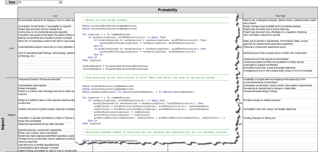 The recent post showed a way how to create a Pivot Table lookalike crosstab with texts in the value area.
However, due to the fact that it was restricted to Excel formulas, the approach came with a couple of drawbacks. Using formulas forces you to define the layout and the size of the crosstab in advance in a static structure. It goes without saying that this considerably limits the usability in real life.
Without VBA, there is no way out. However, some VBA helps to overcome almost all of the disadvantages of the formula based approach. Today’s post is the announced follow-up: it describes how to use VBA to emulate a Pivot Table lookalike crosstab with texts in the value area, as always including the Excel workbook for free download.
The Idea and Concept
The basic idea is a fixed and named cell range on a separate worksheet steering the layout of the crosstab, i.e. the definition which data field goes to which part of the crosstab (value area, rows, columns and filter).
Everything else is done by a VBA routine analyzing the raw data and creating and formatting the crosstab. This routine is executed whenever something changes (data, layout definition or filter).
The crosstab will
- show only the relevant category entries in the rows and columns
- display filter, row and column category entries sorted ascending
- display the texts in the value area as values (no formulas)
- include an automatically created dropdown (form control) as the filter input control
- automatically be formatted
The Preparation of the Workbook
Although we will have the VBA routine to do the laborious work, we still need a little bit of preparation of the Excel workbook:
- Bring your data into your workbook. We are using the same fictitious example data of a project risk list again
- Define a name for the cell range containing the data (“myData”)
- Insert an additional worksheet [Control]. Here is an example screenshot:
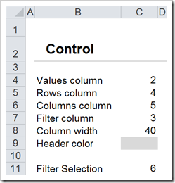
Columns C4:C7 define the layout of the pseudo Pivot Table. The numbers represent the column numbers within our data table. In the example shown above, the data from column 2 of the data table (the risk description) will be displayed in the value area of the crosstab, the data from column 4 (the impact) will go to the rows of the crosstab, column 5 (the probabilities) will be displayed in the columns of the crosstab and column 3 of the data table (the risk type) will be used as the filter. If you want to change the layout of the crosstab later, we do not have to change the VBA code. Instead, we simply change these 4 values. A combination of 2, 3, 4, 5 will bring the risk types to the rows, the impact to the columns and use the probability as the filter.
In cell C8 we define the width of the columns of our crosstab and in C9 we select the fill color for the row and column headers of the crosstab.
Cell C11 stores the actual selected filter.
- Define names for the range B4:C9 (“myPivotTableDefinition”) and for C11 (“myFilterSelection”) in order to be able to address these cell ranges in VBA.
- Finally insert a new worksheet [Pivot Table Risks] and assign a name to the top left cell of our pseudo Pivot Table (“myPivotTableStart”).
The Implementation – The VBA
I think I don’t have a snowball’s hope in hell to describe and explain the VBA code line by line. I did my very best to write readable and comprehensible code (not sure if I succeeded) and added a few comments. Thus, I will restrict myself to a few hints on the general structure of the VBA:
There is only one single module in the workbook containing 2 main functions and 2 main subs:
- The function UniqueItems returns a list of unique items from an array of values
- The function FindPosition does pretty much the same as the worksheet function MATCH. We could use Application.WorksheetFunction.Match(..) instead, but the VBA is faster than calling the worksheet function
- The sub QuickSort sorts an array ascending
- The sub CreateTextPivotTable – this is the main procedure
The sub CreatePivotTable consists of the following main steps:
- Initialize the data structure and transfer the data and the Pivot Table definition from the worksheets to VBA variables
- Delete the existing Pivot Table, unmerge cells, clear all formatting and delete the existing filter drop down
- Prepare the filter: create a list of unique entries in the data field selected as the filter, add the entry “All” and create a filter dropdown on the worksheet
- Detect the row and column headers by creating lists with unique items from the data fields selected for rows and columns
- Loop through all data rows, detect their position within the crosstab (which row / which column) and calculate the number of entries in each field of the crosstab matrix
- Calculate the maximum number of entries per row category
- Write the crosstab to the worksheet
- Format the crosstab
- Update the named formula "myPivotTable"
- Clean-Up (deallocate the data structure)
The code will always delete the existing crosstab and create a new one from scratch. It has to be updated if
- … the data is changed or new data rows have been added
- … the definition of the layout on worksheet [Control] has been changed
- … the user changed the filter by using the dropdown
The update of the crosstab after changing the filter is managed within the VBA code (using .OnSection of the dropdown). In order to make sure that the crosstab is always up to date after changes of the data or the [Control] worksheet, we call the sub CreateTextPivotTable within the event driven procedure Worksheet_Activate of the sheet [Pivot Table Risks]. Every time the sheet is activated, the crosstab will be updated.
That’s it.
The Pros
- It works (well, you expected that, didn’t you?)
- It is easy to implement and easy to use
- The layout of the crosstab can easily be changed
- It eliminates most of the disadvantages of the static formula approach (see the cons described in the recent post)
The Cons
- VBA necessary
- Some preparation of the workbook required, but by far less efforts than with the formula based solution
- Limited to exactly one filter. There is no option for a crosstab without a filter or more than one filter. This would be possible, of course, but I tried to keep it as simple as possible
- Error handling is next to nothing. For instance, the code will not check if it will overwrite data or formulas. There is no warning. You have to make sure that there is enough empty space right and below of the defined start cell of the crosstab
- The layout definition is flexible, but not very user-friendly. A user form with dropdown lists to change the layout and the formatting would be more convenient
The Performance
If you are using a more complex VBA procedure, the performance of the code is always an interesting topic. I did some stress testing. With a relatively small amount of data (150 data rows in the example workbook), the crosstab updates instantaneously. Using a database of 5,000 rows, the procedure takes 0.6 seconds, with 10,000 rows this increases to 1.2 seconds, with 65,000 data rows it takes even 6.4 seconds. Agreed, 6.4 seconds is everything else than a good user experience.
However, I do not think that matters in this specific case: unlike a real Pivot Table, we are not aggregating data. We are simply rearranging it and showing an enumeration in a tabular crosstab. From my point of view this wouldn’t make sense with a large database of 10,000 rows or more. Thus, performance shouldn’t be a problem.
The Download Link
Here is the Excel workbook for free download:
Download Pivot Tables_with_Texts – VBA Approach (Excel 2003 workbook, 121K)
Please be advised that the workbook is Excel 2003 file format, but I tested the code only with Excel 2010. If you encounter any problems with the file using Excel 2003 or earlier, please leave me a comment.
Acknowledgement
Many thanks go to Ulrik Willemoes, who was once more kind enough to spend some of his precious time reviewing my workbook and discussing it with me. As usual, Ulrik provided a couple of very interesting suggestions how the workbook could be improved. Many thanks, Ulrik!
I decided to save one of Ulrik’s best ideas for a follow-up post. So, if you liked this article, please stay tuned. There will be one more post on this topic coming soon.
Comments
77 responses to “Emulate Excel Pivot Tables with Texts in the Value Area using VBA”
Two comments/ideas:
Currently it is not possible to reorder the subcategories within ‘Impact’ and ‘Probability’ in the pseudo.pngvot like you would do in a normal pivot. For instance the order’High’-‘Medium’-‘Low’ makes more sense than ‘High’-‘Low’-‘Medium’. Maybe an idea for a future version..?
I am not sure if this is a problem, but if for some reason your list of data would contain duplicates, they would all be listed in the pivot. Of course, you can say that the list is supposed to contain uniques only, which makes sense in the risk list example. But very often, a datalist also contains some count or frequency per post, like a number of incidents per category. Without complicating things too much, the count could probably be appended to the text string of the values, right? E.g. ‘Insufficient time to plan (10)’. Again, just an idea…
Ulrik,
many thanks for your comment and your excellent ideas. Here are my 2 cents:
1. Reordering subcategories
A very helpful feature no doubt about it. Writing the code to allow and apply a manual sorting is no big deal. A bit more effort is required for creating a nice interactive feature for the manual reordering (e.g. a user form with a category list and up and down buttons to reposition the entries). Furthermore we have to save the manual sort order somewhere in the workbook (in order to keep it, even after the workbook is closed) and the decision what to do if a new category entry was added (e.g. adding this entry to the end of the sort order or setting the sort order back to default). Both things are possible, of course, but require some design, implementation and testing efforts.
A workaround for the time being could be a definition of categories like “1–High”, “2–Medium”, “3–Low”. Agreed, not ideal, but a reasonable workaround.
2. Consolidate duplicates
Another excellent idea. However this needs some considerable changes of the code and – from my point of view – the user should be able to select if he wants to consolidate duplicates or not. I think it always depends on what you are trying to visualize / analyze and the user should have the choice to decide.
Both are very good ideas, thanks for sharing.
However, you didn’t mention your best idea (which we discussed in our email chat 2 weeks ago): Adding a third dimension to the crosstab by coloring the texts in the value area based on another category. In other words: a heat map. I think a heat map is a fantastic idea and would add a lot of information to the pseudo Pivot Table.
Actually, I already started with the implementation of all three ideas, but unfortunately I haven’t made much progress so far. I will definitely publish this as a follow up post, but I have to ask for your patience.
With a larger data set it sppear to stick at 277 rows of displayed data.
Also I noticed when the rows are dates it sorts them by month but does not figure the year into the sort. So you get all the Mays for 2012 2013 and so on, instead of the sorted month day and year.
I can’t reproduce this. As mentioned in the article, I tested the procedure with 65,000 data rows. It is slow, but it is working fine.
The implemented quick sort procedure sorts an array of strings. If you have dates in your raw data, the sorting procedure considers them being strings and sorts them accordingly.
If you want to sort by values, too, you have to implement a more general sorting procedure.
Robert,
As you know, I recently implemented your pseudo pivot on some of my own data and added the discussed heat map. I have also found that using text tooltips that can display additional information on demand, works really well with the text pivot. Just an observation.
Drifting slightly off topic, I am curious whether it is possible to use the Swap routine in your code to swap two defined names?
Ulrik,
many thanks for your comment and another very interesting idea. I know I still owe all of you an update to the pseudo Pivot Table post including all of your ideas and some more. I am still working on the workbook and the article, but I have to ask once more for some more patience.
With regards to your question: you can’t use the Swap sub as it is, but you can write a pretty similar sub to swap 2 named formulas. Something like this:
Sub SwapNames (varFirst As Variant, varSecond As Variant)
Dim strTemp As String
strTemp = varFirst.RefersTo
varFirst.RefersTo = varSecond.RefersTo
varSecond.RefersTo = strTemp
End Sub
Thank you Roberto for sending the link to this site. I had not seen this before. It has some really nice posts. The Excel Hero site has some great members that have sent me links like this. This post is really useful. Very cool.
Christopher
Thank you…Thank you…Thank you…Thank you…Thank you…
Robert,
Your blog is seriously fab… Everytime I have a “How do I” moment with project, excel, reports ect… your blog is my first resource and almost always saves the day.
Thanks for sharing. 🙂
– Sitanshu
This is a really great workbook – just what I needed for analysing some student data comparing past performance to current performance and popping the student names in the table. However I need to be able to reorder rows and columns.
As an alternative, I dont know if there is a way to make a static table which populates with the data so that the Header row is
Current grade B,3c,3b,3a,4c,4b,4a,5c,5b,5a,5c,5b,5a,6c,6b,6a,7c,7b,7a,8c,8b,8a
and the first column is Starting grade B,3c,3b,3a,4c,4b,4a,5c,5b,5a,5c,5b,5a,6c,6b,6a,7c,7b,7a,8c,8b,8a
So that I can get a matrix of students who started at a particular grade and are now at their current grade.
Thanks for the great work. Any help with this request would be very welcome.
Lee,
many thanks for your message and the appreciation. I agree, the sorting of rows and columns isn’t perfect in my solution, even for the example I used (high – low – medium instead of high – medium – low).
Unfortunately there is no easy way out. Here are some ideas, though:
Idea 1: the formula approach
I assume the grades, i.e. the number of rows and columns and the row and column headers are staying the same, so you do not really need VBA. You could also use the formula based approach I described in the previous post. There is one drawback: the fixed number of rows per row header. Roberto Mensa developed an enhanced version which overcomes this and most of the other weaknesses of my formula based approach. Have a look here:
Roberto Mensa’s Formula Text Pivot Table Extreme
Idea 2: rename the entries
You could also slightly change the names of the entries like (1) High, (2) Medium, (3) Low. Might be ok for my example, but certainly no viable way for the grades you want to use.
Idea 3: take out the sorting
You can simply comment out the line in the VBA which calls the QuickSort sub. The “Pivot Table” row and column headers would then be displayed in the same order as they occur in the data source. If you make sure the grades in the data source are sorted as you want them, this is probably the easiest way.
Idea 4: Define the sort order in a worksheet range
You could also use a range on the Control worksheet to define the grade names and change the VBA to get the row and column headers from there instead of detecting a list of unique values from the data source. The VBA code would be shorter and even faster then. One pitfall, though: the definition of the grades would be hardcoded and you have to keep the data source and the definition in sync if new grades are added. However, this shouldn’t be a problem for your workbook, since the grades will probably stay the same over time, won’t they?
I hope this will be helpful.
I ran into a similiar issue before I figured out that you got to define the name range for “mydata”.
I love the spreadsheet, but would it be possible to add a secondary filter?
Salim,
indeed the VBA relies on the defined named formulas like “myData”, etc. exactly the way I described it at the beginning of the post in the section “The Preparation of the Workbook”.
Actually there are a lot of ideas how to enhance this implementation. More filters, more than one data field in row and column headers, elimination of duplicates, a more general sort routine, and so forth. You see: I am having a list…
I always wanted to write an update to this post but couldn’t find the time yet. Maybe later this year. No promise though.
Love it.
Love this spreadsheet, I’m a newbie when it comes to VBA and am trying to cater this to what I need.
I’m trying to add a second values column to facilitate an extra column I have input in column G of the ‘Risk List’ tab.
Am struggling at the moment
Any idea?
Nick,
thanks for your comment.
You do not have to change the VBA, you only have to adjust the named range “myData” to cover the additional data column(s) on the Risk List.
I wonder whether you could replace all that UniqueItem and QuickSort stuff with just a Dictionary object, where you simply add every value – if you’d put “OnError resume next” befor the statement, duplicate values would be simply discarded. To retrieve the list, just use myDictionary.keys.
Interesting idea. I have to admit I do not know much about Dictionary Objects and never used them, but it is probably well worth a try if you could simplify the code. On the other hand, the procedures for getting unique items and the Quick Sort are generic helper routines and I am using those pretty often in my models. The code snippets are there, the code isn’t too long and they are fast enough, I think.
Is there a way to add a sub category in the row field?
Mark,
not with the workbook posted for download above. That being said, it is possible in general (of course), but it requires more complex variable declarations and additional VBA code. In one of my paid projects I have implemented a version with up to 3 dimensions in rows, up to 3 dimensions in columns, up to 10 filter dimensions and even an option to visualize another dimension as a heat map in the value area (different fill colors). The code is way more complicated than in the workbook posted for download above, but it is still pretty fast and working like a charm.
In a nutshell: it is possible, but it takes considerable changes of the VBA code and quite some time to implement it.
I am struggling with the setup of my pivot table. I keep getting the message for “Incorrect Pivot Table Definition”. I am knew to programming in VBA so I am just a little confused as towards what that means and what I have to do to fix that in the pivot table. I have set up a range in the control section just like you did but I am still running into issues. I was hoping you could give a reason why this issue would be occurring. Thanks.
Matt,
thanks for your comment. This error message appears if the definition of the Text “Pivot Table” on the control worksheet is not valid, e.g. you set the rows column value to 5 (column 5 of the data), but your data table has only 4 columns. Or maybe you set one of those control values to 0.
Please be advised that you have to define a dimension for rows, columns, values and the filter. In this simplified version there is no way to e.g. omit the filter or to create a table just with rows, but no columns.
The macro works great until I try to sort by Unit Id than I get the message “The selection contains multiply data values. Merging into one cell will cause the upper left most data only.” How can I fix this?
Mary,
I am sorry, I do not understand your question. I assume you have a dimension (column) called “Unit Id” in your data and this is probably the dimension used as the rows header in the cross tab, right?
I do not understand when you get the error message you described. Did the macro create the cross tab and you try to sort using Excel’s standard sort fnctionality or does this error message appear when the code is still running?
Hi Robert,
In the sample speadsheet you sent I do not get an error message when change the Type from Construction Risks to Design Risks however when change try to do the same using Unit ID. I get the message. I hope this helps to explain.
Thanks again
Mary,
I am sorry, I still don’t get it. I do not understand what you mean by “try to do the same using Unit ID”. If the risk type is set as the filter, you only see a list of all risk types in the drop down plus the option to select “All”. You can’t select “Unit ID” there.
Do you mean you set the ID of the risk list as the filter on the [Control] worksheet? I just tried and it is still working like a charm, although it doesn’t make much sense with this data, because per definition the cross tab always shows exactly one risk unless you select “All”.
I am sorry, I would love to help you, but I don’t understand / can’t reproduce the problem.
Is there anyway that I can send you my spreadsheet?
Mary,
sure, there are “Email Me” links at the top and in the left column of the blog.
The macro works great until I try to sort by “Type” than I get the message “The selection contains multiply data values. Merging into one cell will cause the upper left most data only.” How can I fix this?
Also how do I get column C of the report (your High, Medium and Low) to stop merging.
Any help would be great, I am so close.
Thanks
Thank you it is on its way.
Hi Robert!
Many thanks for the spreadsheet, does exactly what I needed!
However, I took it to the limit, defining “myData” to be all the rows (and 7 columns) that excel 2003 provides (65536).
I ran into 3 issues (the third being another one) and fixed them as follows:
First:
‘ Initialize input data variables
lngMaxEntries = rngData.Rows.Count – 1
varData = rngData.Offset(1, 0).Resize(lngMaxEntries, rngData.Columns.Count)
If Err <> 0 Then
Err.Clear
varData = rngData.Resize(lngMaxEntries, rngData.Columns.Count)
End If
Second:
‘ Initialize the filter variable
varFilterElements = rngData.Offset(1, arrPTDefinition(4) – 1).Resize(lngMaxEntries, 1)
If Err <> 0 Then
Err.Clear
varFilterElements = rngData.Offset(0, arrPTDefinition(4) – 1).Resize(lngMaxEntries, 1)
End If
and third (this doesn’t relate to the max rows problem, however it didn’t work without the err handler):
….
‘ Update named formula “myPivotTable”
ActiveWorkbook.Names(“myPivotTable”).RefersTo = Range(“myPivotTableStart”).Resize(4 + lngDataRows, 2 + UBound(varColHeaders))
If Err <> 0 Then
ActiveWorkbook.Names.Add Name:=”myPivotTable”, RefersTo:=Range(“myPivotTableStart”).Resize(4 + lngDataRows, 2 + UBound(varColHeaders))
End If
best regards,
Roland
Sorry, found some Problem in my Fix, now the header Row is included. If you apply offset AFTER resizing, then excel doesn’t complain about offending its boundaries..
So the two fixes should read:
First:
‘ Initialize input data variables
lngMaxEntries = rngData.Rows.Count – 1
varData = rngData.Offset(1, 0).Resize(lngMaxEntries, rngData.Columns.Count)
If Err <> 0 Then
Err.Clear
varData = rngData.Resize(lngMaxEntries, rngData.Columns.Count).Offset(0,1)
End If
Second:
‘ Initialize the filter variable
varFilterElements = rngData.Offset(1, arrPTDefinition(4) – 1).Resize(lngMaxEntries, 1)
If Err <> 0 Then
Err.Clear
varFilterElements = rngData.Offset(0, arrPTDefinition(4) – 1).Resize(lngMaxEntries, 1).Offset(0,1)
End If
-regards,
Roland
Roland,
I can reproduce your issue. If your data range uses all rows available in the Excel worksheet, the following problem appears:
There are two lines of code initializing the arrays varData and varFilterElements with the data:
varData = rngData.Offset(1, 0).Resize(lngMaxEntries, rngData.Columns.Count)
and
varFilterElements = rngData.Offset(1, arrPTDefinition(4) – 1).Resize(lngMaxEntries, 1)
The problem: the code is trying to offset one row first and resizes the range then. This works well as long as the data range has at least one row less than the data worksheet. This is not the case in your workbook, i.e. VBA tries to offset the range by one row, but there is no row left and the code fails.
Replace the two lines above by
varData = rngData.Cells(2, 1).Resize(lngMaxEntries, rngData.Columns.Count)
and
varFilterElements = rngData.Cells(2, arrPTDefinition(4)).Resize(lngMaxEntries, 1)
This code starts at the second row and the first column of your data and resizes afterwards to lngMaxEntries (65,535).
This should do the trick.
Thanks for the idea; very helpful to know how to use Power Query in another way.
Hi Robert, tnx for your work, I used your table, but it doesn’t go over 150 rows.. May You help me? I have 24000 rows to insert… Thank you so much. (sorry for my basic English XD)
Fortunato,
you have to make sure the named range myData covers all rows of your data. Go to Name Manager and change the “Refers To” of the name myData to cover the entire range of your data.
This worked perfect for me the first time,then I realized that i needed to format the columns as a #, now when I run the macro I only get the filter andthe row header and column header no actual data. What am I doing wrong?
I have adjusted the mydata range to cover all my data which runs from B4 to AM366090
Thanks for your help.
Lynne
Lynne,
I don’t think formatting cells as numbers would be a problem, neither in the data sheet, nor in the cross tab sheet. You can also use a dimension containing only numbers (not texts) on rows, columns or in the value area.
However, there is a limitation in size. Not so much in size of the input data, but in size of the resulting cross tab. In other words, it depends on how many unique entries the dimension in the row header and the dimension in the column header have. The code uses VBA arrays, which can hold a lot of data, but are still limited to a maximum size of used memory. My guess: your resulting cross tab would become too big to handle for the code (a couple of thousand rows and columns) and thus the cross tab can’t be created, at least not with the data structure and algorithm I implemented.
The code doesn’t stop, because of the error handling (On Error Resume Next). You can comment this line out in the code and see where the code stops and which error message you will receive.
I think, it will either stop at the integer counter of the Function Unique Items (i.e. you have more than 32,767 unique entries) or you will receive an overflow error. If it is the integer counter, you can change this variable to type “Long”, but I am pretty sure you will then receive an overflow error.
This is very valuable. Thanks!
Hi Robert, this solution worked great for the data I am analysing. Thank you. You mentioned in earlier comments that the removal of duplicate values is possible, but would require code restructure.
Did you ever get around to taking a look at this? This would be the cherry on the cake for my data!
Robert,
thanks for your comment and your kind words. Unfortunately, no I didn’t. I made some considerable enhancements for one of my clients (like more than one dimension in row and column headers, more filters, heat mapping the data by color, better sorting and many more). Since this was part of a paid project, I am not allowed to share it here. But I never looked into eliminating duplicate values. This wouldn’t be much of a problem, I guess, just a lot of extra coding necessary. Anyway, the code isn’t protected, so if you are familiar with VBA, you could give it a try on your own.
I tried to handle duplicates whilst building the array (amending your code), but got myself into a muddle. Instead, I created a script that runs before your pivot script. This uses the RemoveDuplicates method in excel to create a clean data set in a temporary sheet… I then point your pivot code to this. Adds another ~2 seconds to the run time, but works a treat.
Robert.
I need your help on this Macro to add one more filter, we have filter in My Pivot Table start, how can we add another filter say by another column.
Mahendra,
first you need 2 more parameter cells on the worksheet [control]: one to define the dimension used as the second filter and one for the target cell of the second filter drop down. You also have to define a name for the target cell of the second filter.
Next, you have to adjust the VBA code. I can’t explain every step in a comment. Search for “filter” in the code. Wherever you find it (variable, loop, comment, etc.), you basically have to duplicate the code. E.g. you need the variable varFilterElements twice, you need ddFilterDropDown twice, etc. In the section “Define Filter” you have to do all steps for both filters and so forth.
Sounds complicated, but you have to explore and adjust only 2 subs (UpdateFilterDropDown and CreateTextPivotTable) with a total of only 220 lines of code.
Sorry Robert Tried My level best to fix this but.. was not successful.. if you don’t mind can you please send me Script ?
Mahendra,
unfortunately no. I do not have the time at the moment to implement change requests or enhancements. I am sorry.
No Problem..Thanks
Hi, Robert, I have found workaround to fix my requirement. last one question when we select filter from dropdown immediately macro is not running we have to select another sheet and come back. can we avoid this? I would like to hide datasource
Mahendra,
the macro UpdateFilterDropDown is assigned to the combo box (filter drop down). Every time you use the drop down, the macro is executed and inside this sub the main sub (CreateTextPivotTable) is called. If you have a second filter drop down in your workbook, you have to assign the macro to this one too.
great !! you are genius. I’m alway thinking how to group text by pivot. this is masterpiece that I alway want to find. thank you very much
Hi Robert,
What you described above is exactly what I’m looking for. Any way you can share it?
Thank you,
Dan
Dan,
I am sorry I can’t. As I wrote in my comment above, I developed the code for a client in a paid project. I am not allowed to share it.
What a great idea ! Unfortunately I know zero about VBA, so beyond changing the range to fit my wider and longer table, I struggle to figure out who to customize the table to allow a 2nd column for my row values. In case my question is not clear, let me explain what I’m going to use this for:
I am planning the graduation event for my kids’ school this year. They want a big ball, and there are 10 topics (different areas of responsibility, such as decoration, fundraising, choreography, music, etc). For each topic there are coordination meetings, small information/coordination events, etc. I’ll track everything with this table, shared on my Google Drive. The kids love the idea of each having a “job description”. So I reformatted the table to have the following columns:
1) Index
2) Topics
3) Person
4) Role (such as “Decoration manager”, “Fundraiser Manager”)
5) Meetings
With the tool as it is, I get to choose the “Topic” via the pull-down menu, and the table shows the person on column 1, and I would like to have a “Role” column next to their name, in the grey area, before the data of the “Meetings” that each has to attend gets populated (in the white area).
It looks like this: http://i.imgur.com/dYxfjyX.jpg
I would like to have each kids’ “Job” next to their name.
How should I go about changing the VBA to format the table that way? Thank you for sharing your talent !!!!!!!!!!!
Mike,
several people already asked for the option to put more than one dimension to row and column headers. Unfortunately, this is not possible with the solution posted above. To get what you want, you have to massively change and enhance the VBA code. It is possible, but it is a lot of work. Please have a look at my reply to Mark on April 04, 2013 above.
Thank you for the promt reply, Robert. No chances to resell your previous project, if it fulfills roughly the same purpose? After all, the work is done. 🙂 The PTA may not want to pay for it, but depending on the price tag I might, and use it later on for my house renovation project.
Mike,
unfortunately, no. The code is the intellectual property of my former client. I am neither allowed to share it for free nor to sell it. I am sorry.
Dear Robert,
Is there any way to add one more field in value are. I need wo details and duration against each employee.
Ubair,
not with the workbook posted for download in the article. This version allows only one dimension in the rows, one in the columns and one in the value area. Your request could be implemented, but you have to considerably enhance the VBA code. The code in the workbook is not password protected, so please feel free to change it as you like.
Hi is there a way by which we can have only unique values populated in this template?
Alok,
not with the basic implementation posted in the article above. However, it is possible of course. You would have to adjust / enhance the VBA code to make sure only unique texts are displayed. The VBA project in the workbook posted for download has no password protection, so please feel free to adjust the code as you like.
Thanks a lot, Robert. I will do that. Amazing work though!
i have a table of three columns(group,forms,rights) and i need to get that arranged in the pivot table structured as column – group, row – forms, value- rights(without calculation cell need to display the value of right column)
abilashini,
you can use the example workbook provided in the article right away. Just follow the steps described in the section “The Preparation of the Workbook”.
The template requires a dimension to be used as a filter. I suggest you define one of your dimensions as the filter and set the filter to “All”. Another option would be to change the VBA code and take out all lines of code managing the filtering.
I’m SOOO close to getting what I’m looking for… Unfortunately, I know NOTHING about VBA. My problems are primarily with formatting. My filter box is on my Control worksheet, and my column and row heading are incorrect. Can you help me?
Terri,
sure, send me your workbook by email (see Email
Me-link at the top of the blog) and I will have a look as soon as possible.
Me again. I fiddled around a bit and got the code to work – mainly. Unfortunately, I can’t change the order of the columns, and it appears from your example that you had a similar problem (since your column headings go from “High” to “Low” to “Medium” to “Very High”). Likewise, your row headings go from “High” to “Low” to “Medium”. Is there any way to define the ORDER of the column/row headings?
Ugh. Sorry again. Just read your response to Lee above. I’ll try to figure it out. 🙂
Hi Robert, awesome and elegant solution, and I very much enjoy it.
I have a problem I’d like your opinion on: depending on the filter I put, the amount of rows and columns vary: product x has 4 columns and 3 rows to it, product y 1 column and 1 row. But the other columns and rows remain populated with the earlier called data. This really gives a wrong view. Is there anything I did wrong? Have you encountered this?
best regards,
Stefan
Stefan,
if you did not change anything in the code, it should work, even if products have different amounts of rows and columns. Check it out in the example workbook I posted for download. E.g. set the impact to “High” and the Probability to “High” for all risks of one Risk type on the Risk List sheet and select this Risk Type by using the filter drop down. The Pivot Table will then have only one row header and one column header.
If this isn’t the case in your workbook, I would assume something is wrong with the named range “myPivotTable”. The code clears everything in this range first and then recreates the whole thing. I assume you do not have defined this name in your workbook and that’s why the initial “cleaning part” of the code does not work and the old stuff remains on the sheet.
If this is not the root cause of your issue, you can send me your workbook and I will have a look.
Hi Robert – thanks for your quick response. I indeed did not define the name for the pivot. I’ve updated this, and now it works perfectly. thanks! Great tool. Merry Christmas!
You are a Great Guy… You saved my job. I will include a little icon besides the text message to distinguish visualy the category and will post the code
Again, many thanks!!
I am not sure how to edit this code to get to what I need. Or maybe just manipulate the settings in Control. I want column 1 to be displayed in columns. Column 5 in rows. The values from column 9. I think the issue is filters. I want all the values from column 5 displayed. I am only getting one. I think I just don’t need a filter?
Robert,
I assume you set column 5 as the filter on [Control], too, (cell C7 on [Control])? Simply select “All” in the combo box and you should see all the items.
Hi
Has a second filter been added?
Thanks
Emma,
I am sorry, no. The code is open, though, so please feel free to adjust or enhance the features as you like.