Create Tableau lookalike Chart Tooltips on your Microsoft Excel 2007/2010 Charts
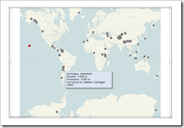 Let’s call a spade a spade: Microsoft Excel’s chart tooltips are lame.
When talking about tooltips I refer to textboxes that appear when hovering over a data point of a chart with the mouse.
Excel’s chart tooltips show by default the name of the data series, the point (e.g. the category) and the values. There is no built-in feature to change anything about them except for turning the tooltips off in Excel’s options.
However, chart tooltips are a great interactive feature. They give the user the opportunity to easily explore the data and get additional information about selected data points on the chart.
Have a look at Tableau as a benchmark. Tableau allows you to display any information in the tooltips (i.e. any given dimension or measure), to format them and to replace the field names by whatever you choose. There is even much more. For instance: my highly esteemed Tableau blogging colleague Andy Cotgreave showed on the outstanding blog of the data studio how to add conditional formatting to tooltips and even how to implement pseudo bar charts inside of a tooltip. Fantastic work, Andy.
Back to Microsoft Excel. Can we do at least something similar in Excel? Let’s stay humble. I am not dreaming of great formatting features or even the fabulous things Andy did with Tableau. I am talking about just some nice and meaningful tooltips displaying more information than the Excel default does. Is this possible?
Yes, it is.
Today’s post shows how to improve Microsoft Excel’s chart tooltips using a textbox and some VBA. As always, providing the Excel 2007/2010 workbook for free download.
The Challenge
A picture (two pictures in this case) says a thousand words:
Microsoft Excel’s chart tooltips are not sufficient, not helpful, sometimes even confusing. In this specific case, I do not care about latitude and longitude. I am much more interested in the name of the mountain, the elevation, the prominence and the first climbers:
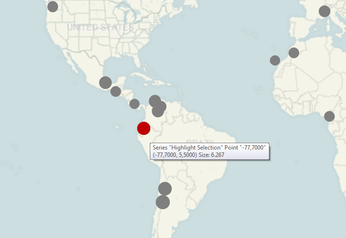
Have a look at the Tableau equivalent:
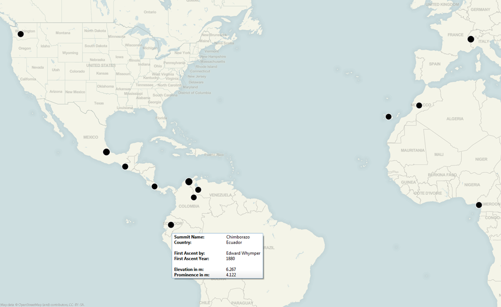
No further comment necessary, I guess.
Here is today’s challenge: provide tooltips in Microsoft Excel as close as possible to what Tableau does by default.
The Idea
The basic idea is inserting a shape object (textbox) to the worksheet and some VBA code to fill it with data and make it visible only if the user hovers over a data point with the mouse.
The Implementation
You may have already noticed that I am referring back to a workbook I already published here on Clearly and Simply: the 50 most prominent summits on earth, a workbook I provided to show how to bluff Tableau Actions with Microsoft Excel.
I decided to enhance this model with better tooltips. The following explanations will refer to the workbook provided back then.
Before starting with adapting your workbook, please be advised that this approach only works properly with Microsoft Excel 2007 or 2010. It will not work with Microsoft Excel 2003 and earlier.
Here is a how-to tutorial to make better chart tooltips with Microsoft Excel 2007 / 2010:
- Create the texts to be displayed in the tooltips
Insert an additional column on the worksheet [Calculations]. Concatenate names of the data fields (strings), values of different columns and a carriage return (CHAR(10)) to one string. The formula looks like this:
=Data!B5&", ("&Data!C5&")"&CHAR(10)&
"Elevation: "&TEXT(Data!F5;"#.###")&" m"&CHAR(10)&
"Prominence: "&TEXT(Data!G5;"#.###")&" m"&CHAR(10)&
"First ascent by: "&Data!H5" ("&Data!I5&")"Simple string concatenation using the ampersand and CHAR. I bet you have done this before.
- Assign a name to the header of this new column to be referred to by the VBA code (“myTooltipBubbleStart” in my example workbook).
- Add a textbox from the shapes menu to the dashboard, format it the way you want to have your tooltips look like and assign a name to the textbox (“myshpTooltip”).
- The VBA – Part I
We enhance the Workbook_Open Sub to make sure the tooltip looks the way we want to. If you are interested, have a look at the workbook posted for download. Nothing special. Just changing color, size and name of the shape.
- The VBA – Part II
We need an additional sub to calculate the points per pixel. I “stole” this piece of code from the fabulous book “Professional Excel Development” by Stephen Bullen, Rob Bovey and John Green. One of the best publications on Excel VBA Development I know. If you are interested in VBA, I highly recommend to buy this book.
- The VBA – Part III
Finally we have to set up a routine to handle the mouse moves. It is a sub called myEmbeddedChart_MouseMove in the already existing class module clsChartEvent. This sub detects the position of the mouse and – if the mouse hovers over a chart point – assigns the defined tooltip text to the textbox and makes it visible. Otherwise the textbox is set back to invisible. If you are interested in the details, have a look at the VBA of the workbook provided for download below.
That’s it. Simple text formulas, a named range, a text box and some lines of VBA code.
The Result
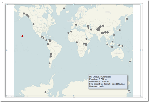
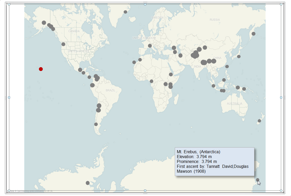
Here is a screenshot of the result. Agreed, not as nice as the tooltips in the Tableau workbook, but – in my humble opinion – better than Excel’s default:
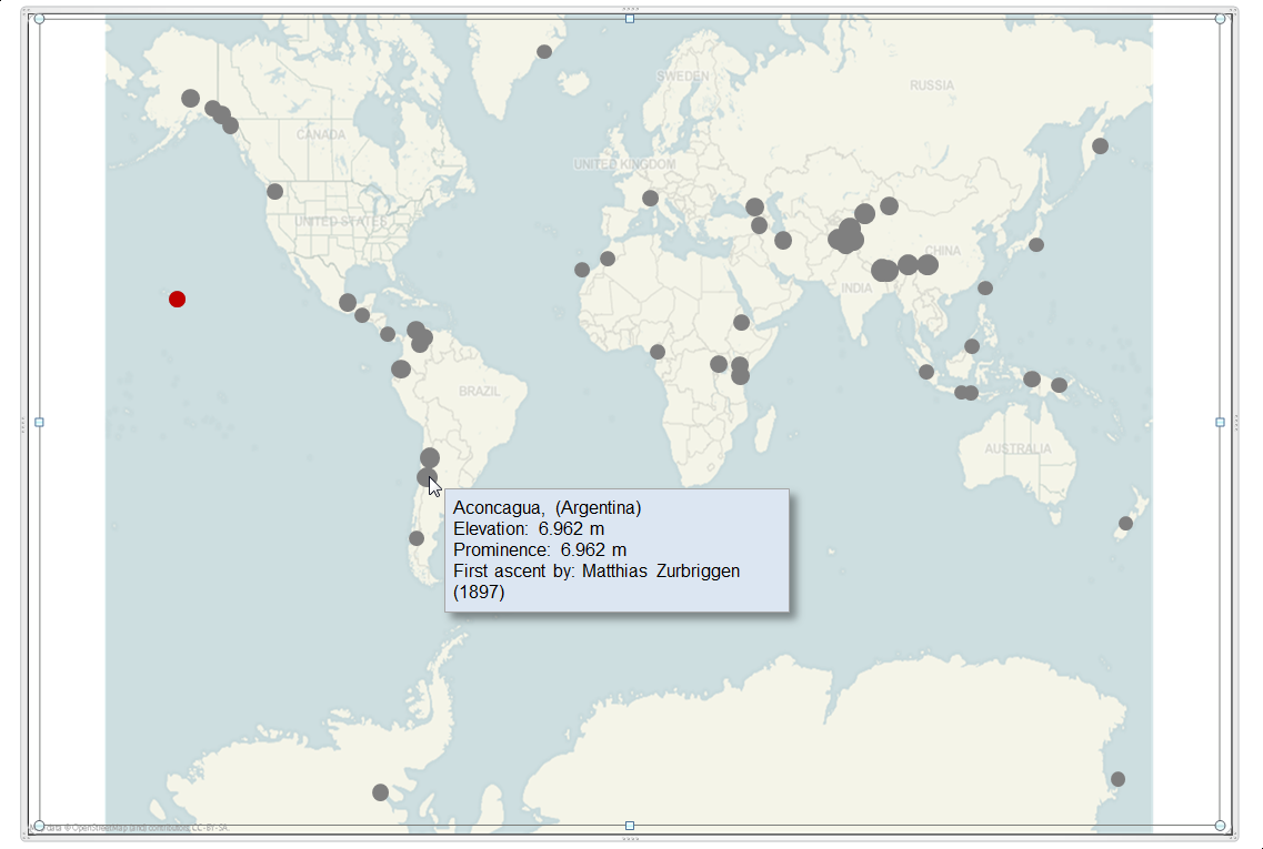 Our VBA code ensures to position the tooltip properly: it usually displays the tooltip to the bottom right of the data point. If there isn’t enough space for the tooltip on the chart, the tooltip is displayed on the bottom left or (like in the following screenshot) on the top left of the data point. This makes sure to always display the tooltip within the chart area.
 The Disadvantages
It is a workaround. Workarounds always come with their own limitations and disadvantages. This one is no exception:
- Unlike the clicking on a data point to update the Google view and the bar chart, the tooltips are not working seamlessly. You have to activate the chart first to make the tooltips working. This is not intuitive and the user has to know this.
- As mentioned above, the approach works only with Microsoft Excel 2007 and 2010. The workbook doesn’t crash if you open it with Excel 2003. You just don’t see the tooltips.
- The approach is based on creating the tooltips in a cell and assigning these strings to a textbox. Formatting options are next to nothing.
A lot of disadvantages, no doubt about it. But it works and it provides better tooltips than Excel’s default without too much effort needed for implementation. Everything else than perfect, but one step up from my point of view.
Let me know what you think.
The Download Link
Here is the workbook for free download:
Download Bluffing Tableau Actions and Tooltips (Microsoft Excel 2007, 468.6K)
More things to come on Excel and Tableau soon.
Stay tuned.
Comments
45 responses to “Better Chart Tooltips with Microsoft Excel 2010”
Very cool. I’m not sure I’d use it with any current projects given the limitations that you described (mainly the fact that a user has to activate the chart – which they have to do even to see the default tooltips). However, down the road, this could certainly come in handy, especially if my presentation was all one “chart” which could stay activated.
Thanks for sharing,
Tom Quist
Great post, and thanks for the links to my blog! I love that you’re taking Tableau’s benchmarks and applying them to Excel. The Action Bluffing is a particularly great solution.
Keep up the great work!
Andy
Haven’t looked at this in too much detail, but I wonder if there’s a way to make this a bit flashier using the Camera tool? Possibly by laying out the Tooltip text across multiple cells and using the Camera tool to capture and display it? Just a thought.
Will,
many thanks for your comment.
A great idea.
Creating a cell range with several rows and columns and capturing the cell range using a camera object for the tooltip gives you a lot more formatting options. You don’t need many changes in the existing workbook.
Instead of a lengthy description how to do this in a comment, I uploaded an example workbook:
Download Better Excel Chart Tooltips with a Camera Object (468.8K)
Thanks again. Very nice idea.
Hi Robert
I had a similar idea using data validation. Here is the link.
http://blog.livedoor.jp/andrewe/archives/50150089.html
I must say using a textbox is better than using a data validation input box.
There is no character limit (at least that I can see) and a lot more formatting can be added. Great idea!
PS The file download link is now http://www.andrewsexceltips.net/Dynamic_Comments.zip
Andrew,
many thanks for your comment(s).
Using the input message of the data validation is a neat idea. As you stated, limited in size and formatting options, but your code is simpler than mine and you do not have to take care of the hiding / unhiding and the location of the tooltip.
Great idea. Thanks for sharing the link and your workbook.
For clarification: Andrew’s comment is referring to the article Tooltips on Microsoft Excel Tables, not to the post above.
Sorry for commenting on the wrong post 🙂
Hi,
Excellent idea….
I’m analyzing scatter diagrams of large test sets (~10k datapoint) and this is great way to quickly see background information for outliers etc.
However, I can not make the tooltops work on a filtered data range as “Offset(lng_argument2,0)” seem to include hidden cells. Is there any way to let offset run over visible cells only? I did play around with SpecialCells(xlCellTypeVisible), but without success.
I’m a VBA beginner, so I apologize if there is an obvious answer to this.
Thanks.
Soren,
thanks for your comment. No worries, as far as I know, there is no obvious answer to your question.
With SpecialCells(xlCellTypeVisible) you are already on the right track. However, SpecialCells does return a range of the visible cells, but it usually is a non-continuous cell range. Thus, you can’t use .Offset or .Cells to directly access the cells with the variable lng_Argument2. You have to transfer the result of SpecialCells to a VBA array and then access the elements of this array to display the tooltip. It is not easy to explain all the details in a comment. If you need further information, please send me an email and I will show you how to do this (email-address see the link on the top left of the blog).
Very nice!
Very Nice!
The main disadvantage seemed to be that the user had to activate the plot before the tool tip would work, however this can be overcome quite easily with a bit of VBA.
Simply position the embedded chart over a range of cells that overlap the chart by a small distance. In each cell you can add the formula:
=IFERROR(HYPERLINK(HoverOverCell(),””),””)
Now, in the VBA Developer environment, create a function called ‘HoverOverCell’ and add some code to activate the chart.
Now, when the user moves the cursor over the chart, they pass over the cells containing the links first, which triggers the function. This means that the chart always become active when the mouse is moved over it.
Adam,
thanks for your comment. You are absolutely right: a User Defined Function in a hyperlink formula can easily overcome the drawback of the technique described above.
For the ones not familiar with this technique: Jordan Goldmeier has a series of great posts on this over at his Option Explicit VBA Blog:
The Excel Rollover Mini FAQ
Finally some shameless self-promotion: I also published a little tutorial here on my blog:
Roll Over Tooltips and Web Actions on a Microsoft Excel Dashboard
Robert, Ive been reading some of your commentary on Excel Pivot Tables with Texts. Ive adapted some of your VBA but have a few questions. Im trying to create 2 row columns to further enhance my filter view. Can you contact me at leese1602@gmail.com I was hoping to show you my pivot table and see if you could show me the next step in the process to create 2. Thanks, Lisa
Lisa,
sure, send me your questions by email (“email me” link at the top of the blog) and I will have look.
Does anyone have the original .xlsm file from the post above? or know how to get the VBA code our of the linked .xlm archive?
Thanks, Tom
Tom,
Excel 2007/2010/2013 files are indeed zipped folders containing XLM and other files. I suppose your browser is set up to directly open these files with Windows Explorer. Just right click on the link, select Save As, save the file to your hard drive, double click on it and the workbook should open in Excel.
Sorry – typo.
The zip file is extracting as an “XML” file structure, not a workbook.
Tom,
there was a typo in my reply as well (XLM should be XML). As I said above, Excel 2007-2013 workbooks are in fact zipped XML-folders.
Don’t extract it using the Windows Explorer, just right click on the link, save the file to your computer and you can open it with Excel by simply double clicking on it.
Thanks Robert – didn’t think to open a .zip with excel. It’s open and I can work through the VBA now. Thanks for your help.
Great and Amazing…
How can be that Microsoft didn’t care to fix the tooltip management?, it’s the same or worse each version (I even have tried to find where to hide tooltips on Excel 2010 and didn’t have a clue…, the older versions there was an easy to find configuration)
I tried your code in an Excel with 64 bits and you will need a change
#If VBA7 Then
Private Declare PtrSafe Function GetDC Lib “USER32” (ByVal hWnd As LongPtr) As LongPtr
Private Declare PtrSafe Function GetDeviceCaps Lib “gdi32” (ByVal hDC As LongPtr, ByVal nIndex As Long) As Long
Private Declare PtrSafe Function ReleaseDC Lib “USER32” (ByVal hWnd As LongPtr, ByVal hDC As LongPtr) As Long
#Else
Private Declare Function GetDC Lib “user32” (ByVal hwnd As Long) As Long
Private Declare Function GetDeviceCaps Lib “gdi32” (ByVal hDC As Long, ByVal nIndex As Long) As Long
Private Declare Function ReleaseDC Lib “user32” (ByVal hwnd As Long, ByVal hDC As Long) As Long
#End If
Tanks a lot.
and (other change)
Public Function PointsPerPixel() As Double
Dim hDC As LongPtr
Darius,
unfortunately I do not have a 64Bit Excel version available, so I didn’t know that.
Many thanks for pointing this out and even providing a solution. This is greatly appreciated.
Hi Robert,
please don’t Warry…my knowledge about Excel is really poor!
I’ve tried to open your attachment…but I’m not able!
In order:
1) I’ve downloaded the .zip file
2) I’ve extracted the content of the .zip file in an empty directory
3) now I find this:
a) [Content_Types].xml (renamed from .xlm)
b) a dir named “xl”
c) a dir named “docProps”
d) a dir named “_rels”
From this point I’m not able to conitnue anyhow in Excel…
Could you please help me?
Thanks in advance
Sergio
Sergio,
as mentioned above, Microsoft Excel files are in fact zipped folders containing XML and other files. Unfortunately, the Internet Explorer changes the file extension from .xlsm to .zip during the download. Simply download the file as posted in the article and change the file extension back to .xlsm in your Windows explorer and you can open the file with Excel.
Sorry Robert!
Finally I got the point. I was reanming the wrong thing. Now, renaming the .zip into .xlms, it works fine!
Thanks again
Sergio
If you want an out-of-the-box solution and you have Excel 2013, you can now benefit from the various apps that are published in the MS Office Store. For example, the yellohcharts app has build in hover over menu for each data point. If you go to https://store.office.com/appshome.aspx and search for the Yellohcharts app, you can try it for free…hope this helps.
Jeroen,
the app looks promising, but – as far as I am concerned – I am never using add-ins or apps providing interactive functionality. I am developing models for other people and forcing my clients to install add-ins before they can use my workbooks isn’t an option. I am using add-ins, of course, but only to increase my productivity, like ASAP utilities or Power Utility Pak. I never use add-in functionality as an integral part of my models.
Having said that, I am sure many people will find your hint very useful and interesting, so many thanks for your comment. Much appreciated.
Robert
Very interested in getting this to work. Downloaded the xlsm file, but when I open it, I get an error in XL 2010 on the Workbook_Open event – it cannot activate Worksheet(1), which is perplexing. WOuld you have any suggestions?
Peter,
I do not know if this is only a typo in your comment, but the correct line of code should read
Worksheets(1)
instead of
Worksheet(1).
Maybe you unintentionally deleted the s?
How to activate the chart to get the sheet working.
Peeush,
activating the chart means that you have to select the chart by clicking on it.
I am having that same problem and my code is below.
AppEventsOn
Worksheets(1).Activate
ActivateSheet ActiveSheet
Application.ShowChartTipNames = False
Application.ShowChartTipValues = False
Error is
Run-time error ‘57121’:
Application-defined or object-defined error
Richard,
the error number indicates that your Excel options are set to disable all ActiveX controls without notification. Change this setting in the Trust Center to enable ActiveX controls and try again.
This is awesome, what codes would I use if the graph is on a sheet tab instead of an embedded chart.
Sorry novice VBA programmer here doing the best I can to reverse engineer. Thanks!!
David,
the technique is possible on chart sheets, too. I am only working with embedded charts, so I do not have the code for a chart sheet available. However, I remember Ajay over at databison published a workbook with tooltips on a chart sheet a couple of years ago:
http://www.databison.com/interactive-chart-in-vba-using-mouse-move-event/
Great, I’ll do my best to follow the instructions. I appreciate the help!!!
Awesome! This helped me a lot with my project.
However, how do you calculate the “changed” coordinates?
Christoph,
the current coordinates of the mouse (when hovering over the chart) are calculated by the VBA sub myEmbeddedChart_MouseMove in the class module clsChartEvent.
If you still need this – set the SpecialCells(xlCellTypeVisible) = a variable of type range and use the longval2 to get the value.
This is great – really useful!
Do you have any suggestion of how best to change the code to work where there is more than one graph on a sheet (from more than one data set)?
I’ve tried making adjustments to use ActiveChart in place of myEmbeddedChart in the hope of then using an if statement with the chart name for the tooltip content but without success.
I should probably say I’m something of a novice with this so any help you can give would be greatly appreciated!
Jo,
please have a look at this example workbook:
Download customizable tooltips on more excel charts (71.8K)
Also, you are commenting on a very old post (from 2010), so I would recommend to also have a look at this article:
Customizable Tooltips on Excel Charts
Thank you, that’s a really clever solution. Need to get my head around how to adapt it to my needs now.
Very much appreciated!
I was hoping to do exactly this – customize the ToolTip on a chart in Excel. This site looked like it would provide exactly what I needed – and it might. But, once I started pulling the thread to actually try to use it, I couldn’t decipher what code was needed where or how to weave it into my Excel file/project. When I moused over locations on the chart in the Excel file provided, I didn’t see any custom ToolTip – so with this series of events, I kinda had to give up.
I think this site is fantastic, and if I had the time to unravel the issues encountered and to figure out what steps I’d actually have to take to make use of it – it would be awesome!
I do wish MS would wake up and actually use their own tools – they’d HAVE to come to the same conclusion that Excel needs some help on ToolTip control!
e,
I agree. The workaround I posted above isn’t self-explanatory. That being said, you are commenting on a post which is 12 years old. There have been some updates in the meantime, so maybe you want to check out this article and see if you can include this into your workbook:
Customizable Tooltips on Excel Charts
This is already 6 years old, too, but probably better since it includes more generic templates.