Spice up your interactive Excel Dashboards with dynamically changing Icons, Pictures or Charts
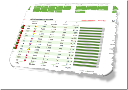
The Excel workbooks which came with two of my recently published posts showed dynamically changing flag icons inside of a dynamic table on an Excel dashboard.
Showcase for Table Slicers on Excel Dashboards
My 2 Cents on the COVID-19 Dashboard by JHU.
The tables visualized data per country and the flag icons next to the country names were automatically adjusted if the user filtered the data, changed the sort criterion or scrolled within the table.
This week I received some feedback on these workbooks and readers asked, if I could explain this in more detail. No sweat: todays post provides a step-by-step explanation of the technique and the according workbooks for free download.
The Requirement and Challenge
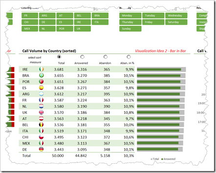
In the Showcase for Table Slicers on Excel Dashboards, one of the views on the dashboard is a table of call volume by country. This table is “spiced up” by displaying flag icons right to the country names. If the user changes the filter(s) with the slicers or the sort order by using the option buttons, the ranking of the countries may (and most likely will) change. It goes without saying that the flag icons only make sense, if they change accordingly:
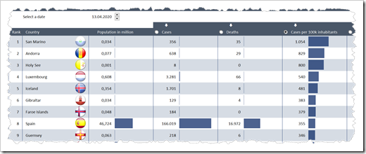
 The workbook coming with My 2 Cents on the COVID-19 Dashboard by JHU showed a similar table by country: again sorting is possible by using the option buttons and the filtering is done by using the spinner to select a day. The challenge is the same: the flag items have to be adjusted according to the ranking of countries in the table. Static icons are not an option.
 The Trick
The trick is a combination of two techniques in Excel:
- Instead of inserting static icons, linked pictures (aka camera objects) are used
- These linked pictures / camera objects are not pointing to a static cell range, but to a named formula. Most often, names are used in Excel to refer to one cell or a cell range only. However, a name can also refer to a formula. Thereby the range, which it is pointing to, can be made dynamic
A Step-by-Step How-to
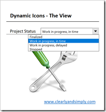
To make this step-by-step easier to follow, I will use a very simple example for this technique: the example will show one out of four icons in a cell range based on a project status the user selects from a drop-down list (a combo box), like this:
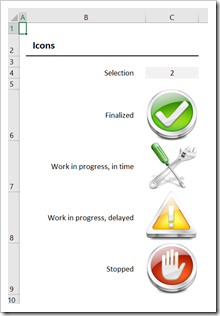
Collect the icons you want to use and insert them on a separate worksheet in Excel. Adjust the row height and column width and resize and align the icons to make it look like this:
 A brief aside: one useful tip you may or may not know: keeping the ALT key pressed during the resizing and repositioning of the icons will make the object snap to the underlying grid of the worksheet. This applies to all objects in a worksheet, by the way, like charts, form controls, freeform shapes, etc. It is probably one of the most useful tips for resizing and aligning objects on an Excel dashboard.
Step 2: Define a Named Formula
Go to the Name Manager (CTRL-F3) and define a new name, like “myStatusIcon”:
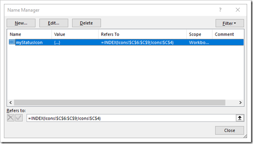 In the “Refers to” bar, you enter the following formula:
=INDEX(Icons!$C$6:$C$9;Icons!$C$4)
This formula will return the row which is defined in cell Icons!$C$4 (which is the target cell of the combo box) inside the cell range Icons!$C$6:$C$9 (where our icons live) . I.e. if the user selects the first item in the drop down, the formula will return $C$6, if she/he selects the last item, it will return $C$9.
Step 3: Insert a Linked Picture
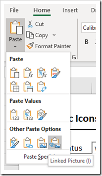
Now go to the sheet where the dynamic icon shall be shown, select any cell range and copy it. Go to Home|Paste and select Linked Picture (bottom right):
 Step 4: Assign the Named Formula to the Linked Picture
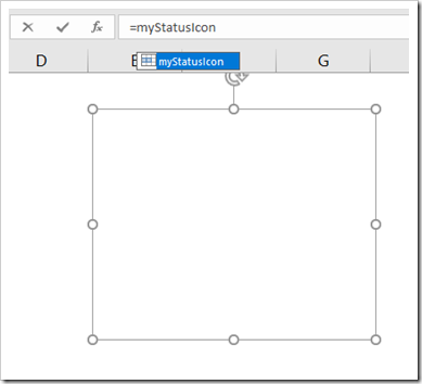
Select the linked picture, go to the formula bar and replace the static link by the Named Formula we defined in step 2:
 That’s it. Four simple steps and we are good to go.
More Icons
If you want to have more icons dynamically changing, you need one linked picture and one named formula for each of them:
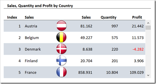 In this example of a scrollable table with five rows, we need 5 linked pictures referring to these 5 formulas:
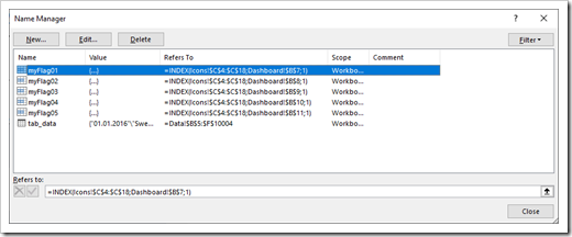 The INDEX function is now referring to the value in the first column of the table instead of the target cell of a combo box as shown in the step-by-step section.
If you have a table with a fixed number of rows (all countries are always shown), you need as many linked pictures and named formulas as you have countries:
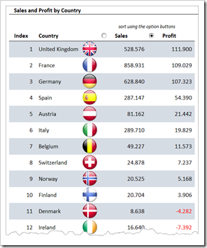 In this table, the user can sort the table by Sales or Profit using the option buttons.
The necessary 15 named formulas look like this:
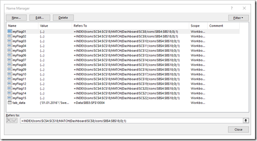 The syntax of the named formulas:
=INDEX(Icons!$C$4:$C$18;MATCH(Dashboard!$C$8;Icons!$B$4:$B$18;0);1)
The row parameter of the INDEX functions is now a MATCH function, returning the position of the country name in the range left to the icons. Please note that the formulas are all identical except for the first parameter of the MATCH function (the value MATCH is supposed to look for, i.e. the country name).
A bit more complicated, but definitely no rocket science. Just laborious work.
Another Use Case: User-Defined Chart Type
Of course, you are not limited to flags or icons. You can display anything in certain cell ranges or sitting on top of them. This could also be company logos or pictures of products, etc.
Or, you can simply let the user decide, which chart type shall be used for visualizing the data, like this:
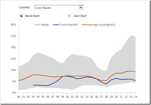 You guessed it: the user doesn’t really change the chart type. He only selects which of two existing charts will be shown on the dashboard. The technique is the same as described above. The only difference: instead of icons, you are pointing to cell ranges where different charts live.
I already used this in a post on this blog, too:
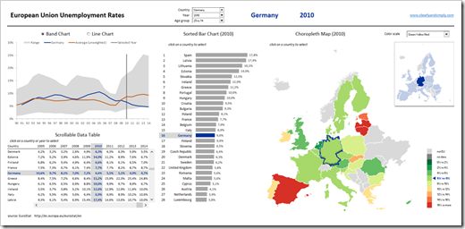 You see: I am eating my own dog food.
Download Link
If you are interested in the 4 Excel workbooks shown above, here is a link to a zipped folder:
Download Dynamic Icons in Excel Cell Ranges
(zipped folder with 4 Excel workbooks 3.3.MB)
Stay tuned.
Leave a Reply