3 Examples of how to use an ActiveX Spreadsheet Control as a Tooltip on a Microsoft Excel Worksheet
 The recent post described how to use an ActiveX Spreadsheet Control as a tooltip on Excel worksheets. At first sight this seemed to be a nifty little idea to spice up tooltips on Microsoft Excel worksheets. In the meantime, however, I had to learn that there is a major pitfall:
The heart of the solution, the ActiveX Spreadsheet Control is part of the so called Office Web Components. So far, so good. The problem is that Microsoft does not ship the Office Web Components with Office 2007 and later anymore. In other words, in a clean, new Office 2007/2010 installation, the ActiveX Spreadsheet Control is not available anymore.
Microsoft still provides the Office Web Components for free download (Office 2003 Add-in: Office Web Components), but there is still a major drawback: if you want to use the described technique, you have to make sure that every user of your workbook either uses Excel 2003 or has the Office Web Components installed.
At the end of the previous post I announced a follow up article with more practical examples using the technique. Knowing now what I didn’t know before, I pondered if this article would still make sense. To cut a long story short, I finally decided to publish it despite the limitation described above. Maybe some of you will still find it interesting and useful.
Today’s post provides 3 different use cases of how to take advantage of the ActiveX Spreadsheet Control in a tooltip:
- a scrollable tooltip
- side calculations within a tooltip
- an improved version of the Summary Card tooltip
As always the articles provides all Excel workbooks for free download.
Example 1 – Details on the selected cell or row in a scrollable list
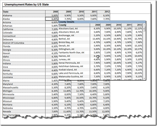
Let’s assume we have an Excel workbook with unemployment rates from 2008 to 2012 by state on the first worksheet and by county on the second sheet. An ActiveX Spreadsheet Control can provide the county details for the active row (i.e. the selected state) in a scrollable tooltip:
The technique for setting up the Spreadsheet Control is exactly the same as described in the how-to post: Interactive Tooltips on Excel Worksheets.
What’s different?
Firstly, you need 2 named ranges for the data (e.g. “myStates” and “myCounties”).
Secondly, the VBA is different. The code in the sheet module (sub Worksheet_SelectionChange) is even simpler than before. However, you need another function retrieving the county details for the selected state (function GetCountyDetails in module modGetCountyData). The code isn’t very complicated. Basically it is working like a filter, i.e. it loops through all counties and returns only those belonging to the current state (selected row).
Here is the workbook for free download:
Download Interactive Tooltip Lookup Details (Microsoft Excel 2003, 670.5K)
Example 2 – Side calculations based on the value of the active cell
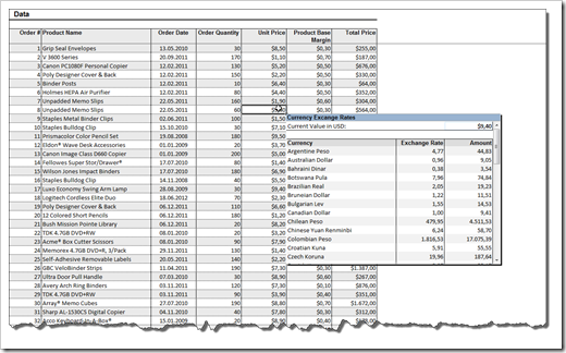
In this example, we have data including some currency values (like prices or margins) and a second worksheet containing the exchange rates for other currencies updated via a data connection to a financial website.
The idea of this use case is to provide a list of other currencies, including the exchange rate and the conversion of the USD amount of the active cell into each currency. The amounts in all currencies are not calculated by the VBA code but rather by a simple formula in the ActiveX Spreadsheet Control (e.g. = B4*$C$1). Hence, the user has also the option to overwrite the USD value in cell C3 of the tooltip (top right) and immediately gets the results for the entered value:
Again we need a second range name (“myExchangeRates”) and a few modifications in the VBA: the code updates the exchange rates in the ActiveX Spreadsheet Control, checks if the active cell has a currency format, writes the value of the active cell to cell C3 of the Spreadsheet Control and finally displays and positions the tooltip:
Download Interactive Tooltip Exchange Rates (Microsoft Excel 2003, 123.5K)
Example 3 – Enhanced Summary Card
The how-to post used the example of a Summary Card in the tooltip, i.e. showing aggregation results of the selected range, like sum, average, maximum, etc.
A helpful little tooltip, but it comes with 2 limitations:
- It does not provide much more information than Excel’s status bar displays already by default
- It aggregates all data of the selected range. This is fine as long as the selected range only covers one column of the data, but it doesn’t make much sense to display e.g. the sum of order quantity and order prices.
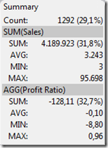
The Summary Card of Tableau, for one, shows the aggregations per measure used in the view:
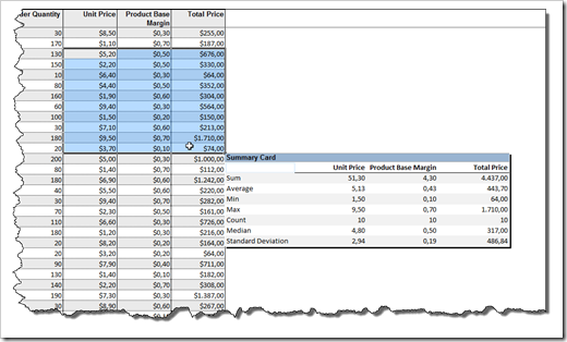
Having said that, we can enhance our Summary Card spreadsheet tooltip to do something very similar, i.e. to show the aggregations in different columns, like this:
The VBA code is a bit longer (55 lines of code compared to 37 in the simple version), but it isn’t really complex.
In a nutshell it loops through the columns of the selected range, performs the calculations column by column, writes it to the according columns of the ActiveX Spreadsheet Control and finally adjusts the viewable range of the tooltip.
There is a lot of room for optimization (e.g. the count is always the same for all measures, so it should be displayed only once above the table, see also the Tableau Summary Card screenshot above), but I am sure you get the idea. For the details please have a look at the workbook:
Download Interactive Tooltip Summary Card Enhanced (Microsoft Excel 2003, 86.5K)
Conclusion
As mentioned in the update at the bottom of the previous post and in the introduction to this article, the entire technique has one major limitation: The ActiveX Spreadsheet Control is not available by default if you are running Excel 2007 / 2010. However, if you are still using Office 2003 or don’t mind to install the Office Web Components, a tooltip including the ActiveX Spreadsheet Control might still be an interesting interactive feature for your models.
Stay tuned.
Leave a Reply