Interactive Tooltips on Excel Worksheets

The Next Level of Tooltips on Excel Worksheets: Taking Advantage of the ActiveX Spreadsheet Control

Tooltips are one of the most helpful features when prospecting large data sets.

We already had a couple of articles talking about tooltips, on charts and on worksheets:

Tooltips on Microsoft Excel Tables

Charts in Excel Table Tooltips

Display all Fields of a Row in large Excel Tables

Better Chart Tooltips with Microsoft Excel 2010

Today’s post is trying to take this to the next level: an interactive tooltip on a Microsoft Excel worksheet. You may ask:

“What the heck is an interactive tooltip?”

What I am thinking of is a tooltip enabling you not only to read additional information but also interact with it. E.g. copy data from the tooltip and paste it somewhere else, do side calculations based on the currently selected data, browse through a longer list of data in the tooltip, etc.

Impossible? No it isn’t. Microsoft provides a very useful ActiveX control which enables us to do exactly this: the Microsoft Office Spreadsheet Control. Today’s post shows how to take advantage of this ActiveX control in order to provide an interactive tooltip on Excel worksheets – as always including the Excel workbook for free download.

The Idea

Microsoft Office / Excel comes with a lot of very interesting and powerful ActiveX controls. One of them is the Microsoft Spreadsheet ActiveX Control. It may sound a bit weird to use a spreadsheet control within a spreadsheet, but it offers a lot of interesting options.

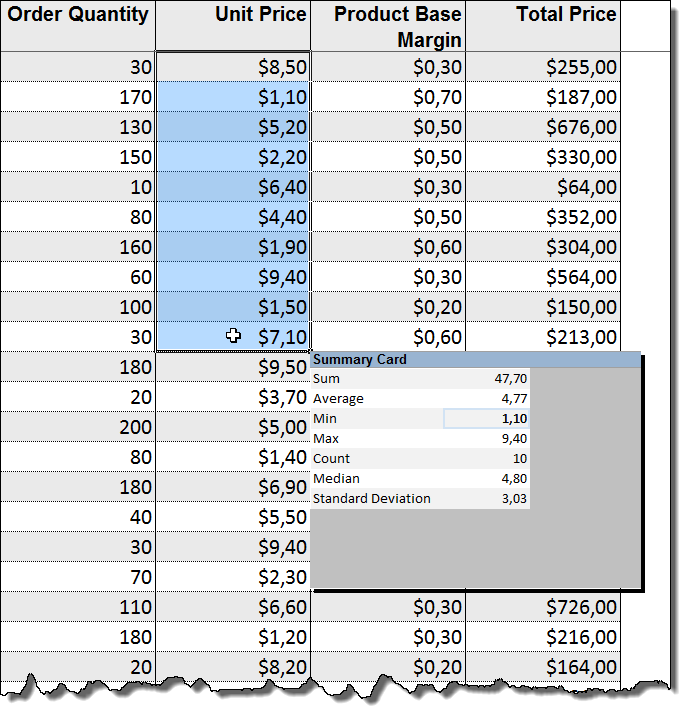
The basic idea of this post is using the spreadsheet control as an interactive tooltip on Excel worksheets. In order to keep things “as simple as possible, but not any simpler” (Albert Einstein), I will describe the idea by displaying a “Summary Card” (see also Tableau Quick Tip #1 – The Summary Card) of the selected range in a tooltip on simple list of data in Excel:

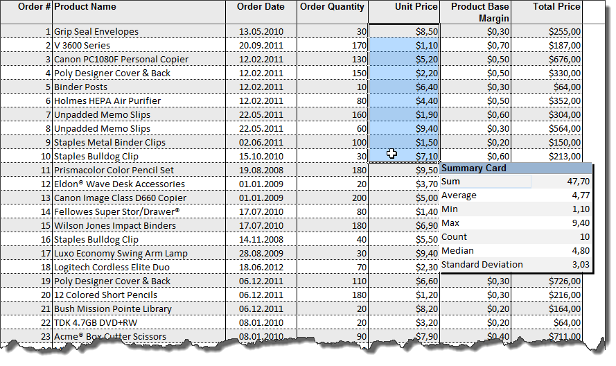The Summary Card displays sum, average, minimum, maximum, count, median and standard deviation of the values in the selected range. Agreed, all of this information (except for median and standard deviation) is available in Excel’s status bar at the bottom right already (in Excel 2007/2010, in Excel 2003 and earlier you only have one of them). However, this is just the first step to show the technique in general. I will provide more useful examples in the next article.

Let’s get started. Here is the how to:

The Step-by-Step Tutorial

Step 1 – Bring your Ducks in a Rows

Insert a data table into a Microsoft Excel worksheet and define a name for the range containing the data (“myData” in my example).

Step 2 – Insert a Microsoft Spreadsheet ActiveX Control

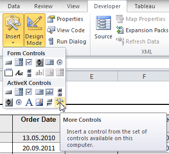
On the Developer tab click on Insert and More Controls:

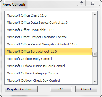
In the following dialogue window scroll down to the Microsoft Spreadsheet 11.0 control and click on Ok:

The cursor changes to a cross. Simply click somewhere on your worksheet and the Spreadsheet Control will be inserted.

Step 3 – Change the Properties of the Microsoft Spreadsheet ActiveX Control

On the Developer Tab click on Design Mode, select the ActiveX Control and click on Properties:

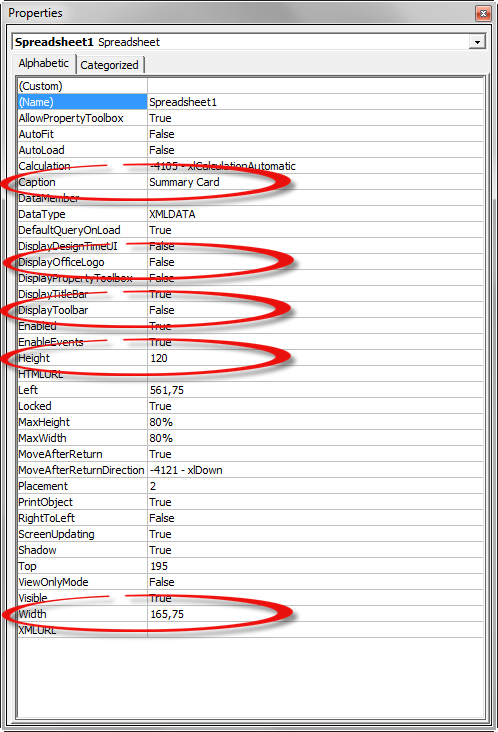You do not have to change much here. Simply define the caption (“Summary Card” in this example), set DisplayOfficeLogo and DisplayToolbar to False and define an appropriate height and width of the control object.

Step 4 – Change the Options of the Microsoft Spreadsheet ActiveX Control

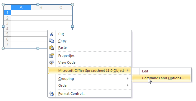
Right click on the control and select Microsoft Office Spreadsheet 11.0 Object and Command and Options:

First tab we go to is Workbook:

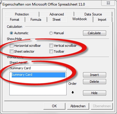Uncheck the scrollbars and the sheet selector, delete all sheets except for Sheet1 and rename the sheet (Summary Card).

Next we go to the Sheet tab:

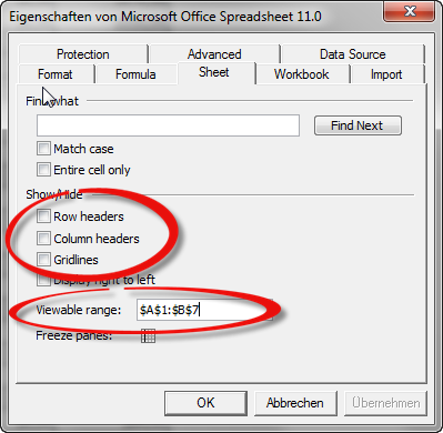Uncheck row headers, column headers and gridlines and define the viewable range. For the summary card example, we need only 2 columns and 7 rows, so we set the viewable range to $A$1:B$7.

Finally we define the column width and row height on the Advanced tab:

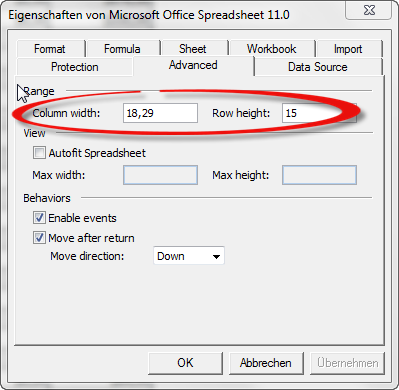Step 5 – Format the Cells on the Microsoft Spreadsheet ActiveX Control

You can use the Format tab in the Command and Options window (see step 4) to format the cells on the worksheet. However it is much easier and faster if you simply create a range on the Excel worksheet, format it as you like (fill colors, borders, number formats, etc.) and simply copy this range and paste it into the ActiveX control. Before you do so, you have to turn off Design Mode on the Developer tab.

Step 6 – The VBA

You guessed it: to make this work we need some VBA. But don’t worry, it is a really small code snippet (2 subs, 37 lines of code). The main part is the event driven procedure Worksheet_SelectionChange. There is one additional function checking if all cells in the selected range are numeric.

Here is what the code does in a nutshell:

1. Check if the active cell is in the data table, i.e. within the defined range name (“myData”)
2. If so, check if the selected range has more than one cell and all cells in the selected range are numeric
3. If so, make the ActiveX control visible, position it at the bottom right of the selected range and insert the results (sum, average minimum, maximum, count, median and standard deviation) for the selected range using the Application.WorksheetFunction method
4. If not, hide the ActiveX control
5. Save the workbook as an Excel Macro Enabled Workbook

That’s it.

The Pros

Well the pros are obvious, aren’t they?

The first one is the ease of implementation: 6 steps and a small piece of code and you are good to go.

Even more important is the interactivity. The ActiveX control is a limited spreadsheet in terms of its functionality, no doubt about it. Having said that, it offers many options you would not expect to have in a tooltip: users can do their own side calculations by entering values into the cells of the tooltip, you natively have the scrolling options for larger tables to be shown, you can easily copy content from the tooltip and paste it somewhere into the Excel workbook or elsewhere, and many more.

Last but not least, the technique offers many possibilities to create a highly interactive and responsive tooltip to prospect data tables. Maybe not suitable for all of your models, but definitely a very interesting option in some use cases.

The Cons

Well, there are not many cons I have encountered so far except for this one: if you change the zoom factor of the worksheet, the ActiveX control resizes too, but the content (i.e. the cell range of the spreadsheet tooltip) doesn’t. You will see something like this:

Not really nice, but a minor drawback in my humble opinion.

The Download Link

Download Interactive Tooltip Summary Card (Microsoft Excel 2003, 73.5K)

Acknowledgements

Special thanks go again to Jordan Goldmeier of the Option Explicit VBA Blog for reviewing my workbook, for his feedback and for encouraging me to write this article. Thanks, Jordan!

What’s next?

As mentioned above, this technique offers a variety of possibilities. Agreed, the Summary Card example does not really take advantage of the interactive features (except for the option to copy the content of the tooltip and paste it somewhere else).

The next post will provide a small selection of examples of what you can do with the ActiveX Spreadsheet control and how to make a really interactive tooltip.

Stay tuned.

Update on Sunday, November 11, 2012 – A
serious limitation

In the cons section of the article I claimed the zooming issue would be the
only drawback of this technique. It turned out that unfortunately this is only
half the story. The ActiveX Spreadsheet Control is part of the so called Office
Web Components. In his comments to this post (see below), reader "Sg" pointed to
the fact that Microsoft discontinued the shipping of the Office Web Components
with Office 2007 and later. This one was new to me. Although I am running Office
2010, the Spreadsheet Control is available on my computer, probably because I
have also installed Microsoft Project 2003.

Microsoft still provides the Office Web Components for free download (Office 2003
Add-in: Office Web Components) and if you install it, I suspect the ActiveX
Spreadsheet should also work with Excel 2007/2010.

However, this is a serious limitation of the technique: you can’t easily
distribute the workbook to other users running Excel 2007/2010. They would have
to install the Web Components first and this considerably decreases the
applicability of the ActiveX Spreadsheet Control for professional Excel
models.