Category: Microsoft Excel

  • Filter Excel Tables by Double Clicking

    How to set the active cell’s value as the filter criteria in Microsoft Excel Tables by double clicking

    Filter - Photographer jercraigs (flickr.com)In a post on the Excel Hero LinkedIn Group Charles asked today:

    “[…] I wish to click on a cell with a purchase order number and have that action filter the list based on that purchase order number.
    What could be a strategy please? […]”

    In one of the answers to Charles’ question, Craig pointed to the most obvious solution: right click and select Filter | Filter By Selected Cell’s Value. Well, I know this is available in Excel 2010, but I can’t tell you no lies: I don’t even remember if this feature was available already in 2003 and earlier.

    Anyway. Although at least Excel 2010 provides a built-in feature for filtering by the value of the active cell, Charles' idea is very interesting and reminded me of a post we had here last year: Sort Excel Tables by Double Clicking.

    The article provided a small VBA code snippet to sort data tables by double clicking into any given column. The technique used back then for sorting can easily be adjusted to implement Charles’ original idea: filter data tables by the value of the active cell after double clicking and remove the filter criteria with another double click.

    The implementation is simple: all you need is to define a name for the range where your data is (e.g. “myData”) and a very small piece of VBA code (24 lines of code) in the event driven Worksheet_BeforeDoubleClick event procedure.

    The code

    • checks if the the user double clicked inside of the data
    • detects the active column
    • checks if the auto filter is set and sets it, if not
    • checks if a criteria is defined already and if so, removes the criteria or otherwise sets the criteria to the value of active cell

    If you are interested in the details, have a look at the workbook provided for download below. If you have any questions, please leave me a comment.

    A simple and effective way of setting / removing filter criteria by double clicking. The technique is not limited to one column. You can also select several columns to filter your data.

    Here is the workbook for free download:

    Download Filter Excel Tables by Double Clicking (Microsoft Excel 2003, 93.5K)

    You can even combine the filtering by double clicking with the sorting by double clicking technique, if you change the VBA to sort only if the user double clicks on the header of a column. A simple IF clause and a combination of the two code snippets will do the job.

    Stay tuned.

  • Interactive Drop Lines on Microsoft Excel Charts

    Display drop lines to both axis of an Excel chart after clicking on a data point

    Ruler - Photographer Auntie P (flickr.com)The previous post (Tableau Quick Tip #4 – Drop Lines) discussed a great interactive feature for exploring large data sets on charts: the Drop Line.

    In fact I like this feature so much that I am not only using in Tableau. If the data is appropriate, I am also providing a similar feature on my Excel dashboards.

    You may ask:

    “Interactive Drop Lines in Excel Charts? Does Excel provide such a feature?”

    Not built-in, but with a few tweaks and a small piece of VBA code, you can easily get to interactive drop or reference lines in Microsoft Excel, too.

    Today’s post shows how to create interactive drop lines on Microsoft Excel charts for different chart types. As always, the article provides the Excel workbooks for free download.

    (more…)

  • Fast Choropleth Map with Enhanced Features

    Enhance a detailed Choropleth Map in Microsoft Excel with additional features

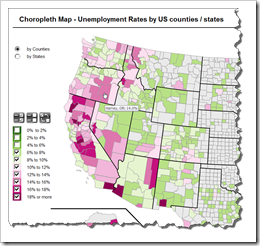
    Choropleth Map with enhanced featuresThe recent article Faster Choropleth Maps with Microsoft Excel provided a faster version of the VBA code to update a detailed Choropleth Map in Microsoft Excel.

    Leonid Koyfman, a faithful reader of Clearly and Simply liked this article. Leonid already contributed his invaluable ideas and insights here before (Excel Multiple Value Filters with Invert Selection). He had a couple of very interesting ideas for the fast Choropleth Map and he is kind enough to share them with us:


    1. Let the user filter the data by value bin and thereby highlight the bins of interest on the map
    2. Show tooltips when hovering over the map to display the name of the county and the unemployment rate in percent
    3. Let the user switch the level of detail: color the map by county or by state

    Today’s article describes Leonid’s enhancements and includes a link to the Excel workbook for free download.

    (more…)

  • Faster Choropleth Maps with Microsoft Excel

    An improved version of a Microsoft Excel Choropleth Map with a better performance for detailed maps

    Choropleth Map US Unemployment by CountyVery soon after starting this blog in 2009 I published a post with a set of Microsoft Excel Choropleth Map templates.  This post is still one of the most popular articles and downloads here.

    A lot of related posts followed and I am feeling very honored that my blogging colleague and France’s data visualization guru Bernard Lebelle of Impact Visuel used 2 of my maps published here on Clearly and Simply in his great new book “Convaincre avec des graphiques efficaces”. Bernard was kind enough to point his readers to my blog in the book. This is much appreciated. However, he should have heaped the praise on Tushar Mehta, who invented this technique. I only “stole” Tushar’s idea.

    Tushar’s approach works great and I know from comments and emails that a lot of my readers have used it with great success.

    There is only one minor drawback with Tushar’s approach: the performance decreases considerably when using it on a map with a lot of shapes, like the US by Counties.

    Today’s post tries to heal this. It discusses how to considerably improve the performance of a detailed map. The article describes the original approach, the optimization potential, the improved implementation and – as always – provides the Excel workbook for free download.

    (more…)

  • Microsoft Excel Check List Template

    A Microsoft Excel template for a structured Checklist with the option to check and uncheck by double clicking

    Checkmark / Photographer: Allen Mc Gregor (flickr.com)Unfortunately my blogging activities slowed down to a crawl during the last few months and I left you waiting for new posts far too long already.

    Be assured that this site is not dead. I will revive the blog during the next weeks and I am already working on a couple of new articles.

    For one of the planned next posts I needed a checklist template. There are tons of Microsoft Excel and Microsoft Word examples available for free.

    However, I couldn’t find a checklist template I really liked. Formats are always easy to change, but I was particularly looking for a checklist providing a convenient way to change the status of the checklist items. Furthermore it should be easy to use and easy to maintain. Some of the templates I found simply expect to type in an X (or something similar) to check an item, some are working with data validation lists, some have form control checkboxes. The one that came closest to what I was looking for is provided by my good friend Daniel Ferry, the Excel Hero here: Excel Dynamic Checkmark. Already pretty close to what I was after, but since it did not fulfill all of my requirements, I decided to create my own.

    Agreed, today’s post is a bit off topic regarding the focus of this blog. It has nothing to do with data analysis, data visualization or dashboards. However, a nice Excel checklist template is always a useful thing to have in the toolbox.

    With today’s article I am trying to kill two birds with one stone: to show a sign of life and to share my little checklist template with you.

    (more…)