Visual Workbook Navigation with a Chart Carousel

A Carousel of Charts as a visual and interactive Navigation Control for Microsoft Excel Workbooks

726 words, ~4 minutes read

If your Excel workbook has many output worksheets, you should provide your users with an option to facilitate the navigation within the model.

Sure, the user always has the option to right click on the arrows left to the first tab and select any worksheet from there, but this requires that she/he exactly knows where to find what.

It is best practice to give the users guidance regarding the content of your model and to enable them to easily navigate to the sheets they are most interested in. Usually, you insert an extra worksheet containing a list of all tabs with hyperlinks or buttons to quickly navigate to those sheets.

You are interested in something more visually compelling? If so, you came to the right place. Today’s article provides a visual workbook navigation control with a chart carousel dynamically displaying the content of the relevant sheets. The user can easily browse through all views, select the desired one and get to the view with one mouse click. As always, the post comes with an example workbook for free download.

The Inspiration

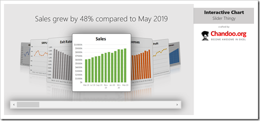
A couple of weeks back, my good friend and long-time Microsoft Excel MVP Chandoo published an innovative and interesting post about how to create an interactive chart slider in Excel: How to make an Interactive Chart Slider Thingy

The Idea

I liked Chandoo’s idea a lot and I thought this could also be used for a visual and interactive workbook navigation control. Here is a screenshot of what I have come up with, based on Chandoo’s solution:

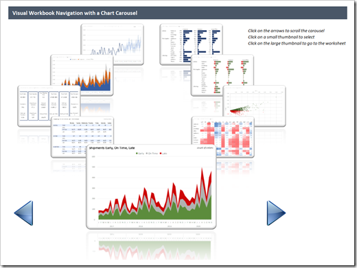On a dedicated navigation worksheet, linked images to 9 different views (worksheets or dashboards) in the workbook are shown as a carousel of thumbnails. The larger thumbnail at the bottom of the carousel serves as the “currently selected view”.

You can

• click on the Left Arrow or Right Arrow icons to change this selection to the view at top left or top right of the large thumbnail
• click on one of the 8 smaller thumbnails to directly select this view. The arrangement of all views will be adjusted accordingly
• click on the large thumbnail to navigate to the worksheet where this view lives

The Implementation

My implementation is a bit more complicated, but still based on Chandoo’s ground work.

Here are the main parts of my solution:

• Just like Chandoo, I am using linked images. I have more views (9 instead of 7) and they are arranged as a carousel, but that’s all
• The linked images are named “shp01”, shp02”, etc. The larger image at the bottom is the first one (shp01) the others are named clockwise
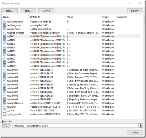
• Names are defined for all ranges of the 9 worksheets where the charts / views live. E.g. the name myView01 refers to =’view 1′!$B$4:$L$17, where [view 1] is the name of the first output sheet
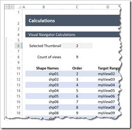
• On worksheet [calculations], cell C6 contains the currently selected view, i.e. the one which is shown in the large linked image (shp01):

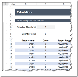
• The small table (range C11:D19) beneath this central model parameter is the heart of the solution. It maps the defined target ranges to the shape names. The formulas are as simple as can be. If you are interested, please have a look at the workbook (download link see below).Here is a screenshot of the mapping table if the second shape was selected:
• The images on the worksheet [navigator] are then linked to 9 additional Named Formulas called myTN01, myTN02, etc. These Named Formulas fetch the target range name from the mapping table and turn it into a range using the function INDIRECT:

• Finally, a very simple piece of VBA code is assigned to all shapes on the worksheet [navigator] respectively to the arrow icons. It is really simple VBA code and only 26 lines. If you are interested, please download the workbook and have a look.

Acknowledgement

Many thanks go to my friend Chandoo. You are always thinking out of the box and this makes you a fantastic source of inspiration for all of us. Thank you very much!

Download Link

Here is the Excel workbook for free download:

Download Visual Navigation w/ a Chart Carousel (zipped Excel workbook, 3.8MB)

Stay tuned.