Gapminder Replica in Microsoft Excel

A Gapminder-lookalike animated chart in Microsoft Excel, based on the generic Motion Chart Excel Template
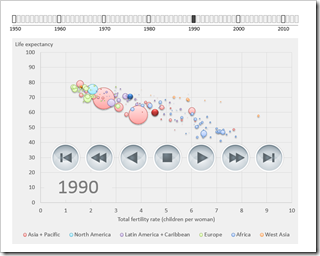
Gapminder Replica in Microsoft Excel

The recent article Motion Chart Excel Template provided a generic template for a motion or animation chart in Microsoft Excel. The examples in that post visualized episodes of the Italian cartoon series La Linea (La Linea article on Wikipedia).

Today’s article will put the motion chart template to a more serious, business like use: a Gapminder replica in Microsoft Excel.

For those of you who do not know Gapminder: Gapminder is a data visualization software to animate statistics. It was originally developed by Prof. Hans Rosling and his team and Prof. Rosling presented it in this famous TED talk:

Hans Rosling shows the best stats you have ever seen

Today’s article rebuilds this data visualization and animation in Microsoft Excel using exactly the same metrics. As always, the Microsoft Excel workbook is provided for free download.


The Features of the Dashboard

I recently read this great quote by @IconFinder:

“A user interface is like a joke. If you have to explain it, it’s not that good.”

Well, if I would be sure my visualization and the interactive features would be fully self-explanatory, I shouldn’t need this section. But I am not.

So here are a few hints what you can do with this dashboard:

  • The heart of the dashboard is the Bubble chart on the left side. Like the example presented by Prof. Hans Rosling, it visualizes fertility rate in children per woman on the horizontal axis, life expectancy in years on the vertical axis and the countries as bubbles. The size of the bubbles represent the population of the countries. The bubbles are color coded by continent and the selected 3 countries to be highlighted (see below)
  • The rectangles above the chart visualize the time line and the current year and let you select one specific year by simply clicking on any given rectangle
  • With the play buttons at top right you can start and stop the animation, move forward or backwards, go to the first or last year. You can also choose whether you want the animation to loop with the checkbox, i.e. start at the beginning after reaching the last year in the data
  • In the highlight section beneath the play buttons you can define 3 countries with the drop down lists to be highlighted in different colors and you can use the “Show highlighted countries only” checkbox to only display these 3 countries in the chart
  • The table right to the drop down lists shows the measures of the highlighted countries and visualizes the maximum value of fertility rate and life expectancy with a grey fill color
  • In the “Filter by region” section you can select which continents shall be displayed
  • Like in the highlight section, the table shows the metrics (weighted averages of fertility rate and life expectancy, sum of population). Again, the maximum values are marked with a grey fill color

The Implementation

Calculations

In order to keep the calculations as simple as possible, I added a unique identifier to the data: a combination of country and year makes it easy to find the relevant data.

Most calculations are pretty simple formulas, mainly INDEX, MATCH and IF. Nothing new under the sun. The most relevant calculation for the chart is the column “Filter” on the calculation worksheet which defines which countries will be displayed in the chart and which won’t.

The only complex part are the array formulas to calculate the weighted averages. The formulas are creating a vector with the product of the measure and the population for each relevant country and year, sum this vector up and divide the result by the sum of population in the given continent. They may look complicated but as soon as you know how arrays work in general, they should be easy to understand.

Bubble Chart

The chart is a standard Excel Bubble chart with one data series for each continent, one for each highlighted country and a scale dummy series to keep the size of the bubbles in relation to the population of all countries in the data, even if a filter is active, i.e. not all countries are displayed.

Animation

Not much to say here, I guess. The workbook is based on the generic Motion Chart Excel Template. If you are interested in the details, please have a look there. The animation control parameter in the Gapminder replica is the year (of course).

The Interactive Time Line

This is the only part of the workbook which needs additional VBA code. Each of the rectangles has a certain shape name (e.g. “Rectangle_1950”) and the sub ClickOnTimeBox is assigned to each rectangle. The sub identifies which rectangle has been clicked on (using Application.Caller), changes the value of the current year, updates the fill colors and stops the animation. Only 2 subs with only 5 lines of code. This should be easy to understand.

The Download Link

Here is the workbook for free download:

Download Gapminder Excel Replica (Microsoft Excel 2007-2013, 824.5K)

Stay tuned.

Comments

36 responses to “Gapminder Replica in Microsoft Excel”

  1. sam Avatar
    sam

    Work of Art Robert….Thank you so much for sharing….

  2. Paul DeVito Avatar

    Beautiful. Thanks, Robert. You probably already know this, but just FYI, this doesn’t work on Excel for Mac 2011.

  3. Robert Avatar

    Paul,
    you are right. The code in my workbook uses the Windows function Sleep for the delay in milliseconds and this function isn’t available on Mac.
    You could either delete the declaration of Sleep and all calls of the function, but then the speed of the animation cannot be controlled anymore (e.g. forward and fast forward would be the same). The other option is to use Application.Wait instead of Sleep.

  4. online excel training Avatar

    Cool! Looks very promising. Thanks for sharing.

  5. Liam Avatar
    Liam

    Awesome. How would you go about changing the years to say months?

  6. Robert Avatar

    Liam,
    adjusting the workbook to another timeline (more or less years or months instead of years) isn’t too complicated for most features. Basically you have to change the ID (combining the country and the year) and change the values of myMin and myMax to fit to your new timeline.
    Having said that, changing the rectangle timeline above the bubble chart takes more time. You would need more or less rectangles with a certain naming convention (e.g. “Rectangle_Jan” instead of “Rectangle_1950”), change the labels of the “axis” beneath the rectangles and adjust the VBA code which extracts the year or month from the freeform name. Not really complicated, but some changes necessary.

  7. NARAYAN Avatar
    NARAYAN

    Hi ,
    Thanks for sharing.

  8. Eirik Avatar
    Eirik

    Great chart – thanks for sharing. Any idea how to create the ‘trail’ for any particular country series over time?

  9. Robert Avatar

    Eirik,
    no sweat. Have a look here:

    Download Gapminder Excel Replica with Trails (843.9K)

    You can select any of the highlighted countries to show the trails over time.
    Same techniques as used in the original workbook, just 3 more data series in the chart and 3 more checkboxes.

  10. Elle Avatar
    Elle

    What’s the recommendable version of Microsoft Excel for this?

  11. Robert Avatar

    Elle,
    I developed the workbook using Excel 2013, but it should work with Excel 2007 and 2010, too. If you replace the IFERROR statements on the dashboard by an IF(ISERROR(…)) construct, it should even work with Excel 2003 and earlier.
    It doesn’t work on a Mac, though. See also my reply to Paul above.

  12. Juan Avatar

    Hi Robert
    Could it be possible to edit the chart and put my own info?
    Like if i want to put how many money did i earn deppending on where i was working through time?
    TIA

  13. Robert Avatar

    Juan,
    the workbook is open, so you can put in any data you like. Just have a look at the data and the calculation worksheet and see how the data is structured and what you may have to change.

  14. Juan Avatar

    Thank you Robert!
    There is a sheet called Data, i changed some countries(like spain to spanish) but when i want to select it on the highlights (on the dashboard sheet) it dosent appear.
    I’d saved the document, closed it, and opened it again, and nothing
    What im doing wrong?
    TIA

  15. Robert Avatar

    Juan,
    you also have to change the names of the countries on the sheets calculation and control.

  16. Juan Avatar

    Ok, thank you for your patience haha!
    Last one i swear!
    Can i add a country or i just can edit it?
    TIA

  17. Robert Avatar

    Juan,
    you can also add countries, but you have to
    1. enhance the list of countries on the worksheet control and add the name(s)
    2. enhance the calculation range on worksheet calculation and add the names and formulas
    3. make sure the data sources of the chart are covering the correct ranges on worksheet control
    As long as you take care of this, you do not have to change anything in the VBA code.

  18. Juan Avatar

    Really this is the last one….
    Just kidding
    Thank you !!
    Merry Christmas

  19. Mark Avatar
    Mark

    This is great. Thank you. Can I change the type of chart from bubble to a line chart or any other type chart?
    Mark

  20. Robert Avatar

    Mark,
    technically: yes, you can use another chart type. Whether a line chart would make sense depends on how your data looks like, what you want to display and what you want to animate.

  21. Arun Singh Avatar

    Hi robert, I don’t know VBA atall, but can you show with an example how to change parameters such as timeline. I am trying but not been able to go further. Kindly help

  22. Arun Singh Avatar

    Hi robert, I don’t know VBA atall, but can you show with an example how to change parameters such as timeline. I am trying but not been able to go further. Kindly help

  23. Robert Avatar

    Arun,
    in the example workbook provided above, there is a named range called myCurrentValue (cell C10 on worksheet control). The VBA routines IncreaseCounter and DecreaseCounter increase or decrease this value with a delay in milliseconds passed to these procedures by the parameter lngWait.The VBA routines Forward, FastForward, Backward, FastBackward, ForwardToEnd and BackToStart then call one of these two routines to in- or decrease myCurrentValue as desired. These routines are assigned to to the play buttons on the dashboard and will be executed if the user clicks on one of the buttons. VBA increases or decreases the value of myCurrentValue and all calculations in the workbook are based on this value.
    I hope this sheds some more light on the technique.

  24. Arun Singh Avatar

    Hi robert, Thanks for your reply, I want to create a personal project for data with last 10 years, so I can develop all the necessary calculation in excel but how can I change my Time line from “1950 – 2013” to say “2007 – 2017”.
    Can you help me with this as I tried to make this work by changing “Mymax” and “My min” values but didn’t get success.
    Kindly help with some example.

  25. Robert Avatar

    Arun,
    I will send you a version for 2007 to 2017 by email in a few minutes.

  26. Robert Avatar

    Arun,
    I just noticed that TypePad is not providing me with the email addresses of my commenters anymore. Can you send me a short email (click on the “Email Me” link at the top of the blog) and I will reply with the workbook from 2007 to 2017. Thanks.

  27. bish Avatar
    bish

    Hi I get an error when I run:Run-time error ’13’:
    Type mismatch

  28. Bish Ashleigh Avatar
    Bish Ashleigh

    I am running Excel 15.31 for Mac and I get Run-time error ’13’:
    Type mismatch

  29. Robert Avatar

    Bish,
    please have a look at my reply to Paul (third comment from top).

  30. Arun Singh Avatar

    Dear Robert, Thanks for your support, I am just checking if you have had emailed me the sheet. If not, can you share it on "[…]"
    Regards
    Regards
    Dr. Arun Singh Rana (PT)
    || Cell: […] ||

  31. Robert Avatar

    Arun,
    I will send you the workbook in a minute.
    PS: I edited your comment and took out your personal information to avoid spam in your inbox and unwanted calls. I hope I acted in your best interest.

  32. Leroy Avatar
    Leroy

    Hi Robert,
    I’m excited to find your post as I have been building my own version (struggling with a few feature though). When I download the zipped file it appears to hold XML Documents and I can’t access anything. Should the files come up showing excel symbols?
    Regards

  33. Robert Avatar

    Leroy,
    since version 2007, Microsoft Excel files are actually zipped folders including XML and other files. If your Internet browser opens Windows Explorer when clicking on the download link, right click on the link instead and select “Save Target As” to download. If you are using Microsoft’s Internet Explorer or Edge, the IE/Edge will change the file extension from .xlsm to .zip during download. Simply change the file extension back to .xlsm and you can open the workbook with Excel by double clicking on the file.

  34. Way Avatar
    Way

    Hi, how do i change the timeline to 2011 -2017?

  35. Robert Avatar

    Way,
    here are the main steps:
    1. Adjust the data to have only data from 2011 to 2017
    2. Make sure the combinations in column ID (Country/Year) on the data sheet are adjusted, too
    3. Adjust the values of myMin (=2011) and myMax (=2017) on the control work-sheet
    4. Set the value of myCurrentValue to 2011 (as a starting point)
    5. Rename the rectangles on the dashboard: Rectangle_2013 becomes Rectangle_2017, Rectangle_2012 becomes Rectangle_2016 and so forth
    6. Delete all not necessary rectangles on the dashboard (Rectangle_2006 and earlier)
    7. Adjust the axis labels of the rectangles
    8. Resize / reposition the rectangles as you like
    This should do the job.

  36. Kenneth Avatar
    Kenneth

    Arun,
    May I ask if you we’re able to make the above file work in Mac?

Leave a Reply to Mark Cancel reply

Your email address will not be published. Required fields are marked *