Marimekko Charts in Microsoft Excel

A VBA based Microsoft Excel Template to create a Marimekko Chart aka Matrix Chart aka Mosaic Chart for free download
marimekko #2 - Photographer: 4WheelsofLux (flickr.com)A Marimekko or Matrix or Mosaic Chart (called Marimekko hereafter) is a combination of a 100% stacked column chart and a 100% stacked bar chart combined in one view. It works like a 100% stacked column chart, but additionally the width of a column is proportional to the total value of this column.

Microsoft Excel does not provide a built-in chart type for Marimekko charts, but there are several workarounds available to accomplish this. For instance, Jon Peltier shows in his article Marimekko Charts how to turn a combination of a stacked area and a line chart into a Marimekko chart. My friend Chandoo, Conditional Formatting aficionado he is, uses the cell grid, formulas and cell value based formatting rules to create a pseudo Marimekko chart in his post Market Segmentation Charts using Conditional Formatting. Of course there are also a couple of other blog posts on this topic and also commercial Add-ins available.

Although Jon’s and Chandoo’s solutions work well and are available for a long time already, I decided to add my 2 cents with another approach: a VBA based solution creating a Marimekko chart made up of freeform text boxes. The main advantage: reduced set-up time and more flexibility, if the number of rows and columns of the Marimekko chart changes.

Today’s article provides a VBA based solution to create a Marimekko chart in Microsoft Excel and explains how to use and customize the template to suit your requirements. As always, the workbook is available for free download and the VBA code is without password protection.

The Approach

Instead of tweaking a built-in Excel chart type like Jon or using the cell grid and Conditional Formatting like Chandoo, this template will use VBA to create a Marimekko chart made of freeform shapes (text boxes). So, it isn’t a real Excel chart: it rather is a group of textboxes looking just looking like a chart. This is exactly the same basic idea and approach my friend Fabrice Rimlinger uses for his great Sparklines for Excel.

In a nutshell, the code to create the Marimekko chart

  • imports the data into a VBA array,
  • calculates totals and percentages,
  • adds text boxes (freeform shapes) to the worksheet,
  • changes the size of the textboxes based on the single and total values and the size of defined range where the chart shall be displayed,
  • moves the textboxes to the right position
  • changes the text in the textboxes,
  • formats the textboxes
  • and finally inserts row and column headers, row and column totals and a grand total

Before it does all that, it destroys what’s there already. In other words, every time the chart is updated, the algorithm deletes everything and recreates the whole thing from scratch.

Well, this sounds as if the approach would come with some serious performance problems. However, the performance is actually still acceptable from my point of view, even for an interactive dashboard. The code needs ~0.4 seconds to create a 10 rows / 10 columns Marimekko chart. For 25 rows / 25 columns, the algorithm needs  ~1.3 seconds. As I said: still acceptable, I think.

Truth be told, a 100 times 100 matrix takes almost 31 seconds, but honestly: Do you think you will still see something in a Marimekko Chart with 10,000 data points?

The Template

The Microsoft Excel template (download link see below) for creating a Marimekko chart is VBA based, but it is a stand-alone workbook, i.e. you do not have to install an add-in or anything else. All you need is the Excel workbook and to enable the execution of the macros in your security settings or when opening the workbook.

The template consists of three worksheets:

Marimekko

The display of the chart (which is in fact not a real Excel chart):
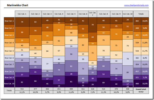
Marimekko Chart

Data

The underlying data, i.e. a crosstab with row and column headers and positive numbers in the value area, similar to a simple Pivot Table: Worksheet [Data]

Control

The definition of the color scheme used to color encode the chart:

Worksheet [Control]

How to use this Template?

You have two options:

Option 1: Use it as it is

Use the workbook as it is and simply paste in your own data into the crosstab on the worksheet [Data]. The chart will be updated every time you activate the sheet [Marimekko].

Option 2: Transfer it to your own workbook

If you want to create a Marimekko chart in one of your own Excel workbooks, you have to transfer the VBA code and to define the required named ranges. The following steps are necessary:

  1. Open your existing workbook and the Marimekko template
  2. Go to the VBE and click on the module modMarimekko of the template and drag and drop it to your own workbook.
  3. Copy the code from the worksheet object Marimekko and paste it into to the sheet object of your workbook where you want to have the chart displayed. This way, the chart will be updated every time you activate this sheet
  4. Define the required named ranges in your workbook:
    • myData: this named range covers the crosstab with the data to be displayed, but without row and column headers. Row and column headers have to be adjacent left and above to the data
    • myChartArea: this is the cell range where the chart will be displayed. The VBA code requires myChartArea to have at least 3 rows and at least 3 columns. The range can cover as many rows and columns as you like, but at least 3
    • myColorScheme: this is the range where fill color and font color of the Marimekko chart are defined. Select a range in your workbook, set the fill and font colors of the cells as you like and assign the name myColorScheme to this range. myColorScheme needs to have at least as many cells (colors) as you have rows in your data (one color for each row)
    • If not done already, save your workbook as a Macro-enabled Excel workbook

How to customize the Marimekko Chart

The options to customize the Marimekko Chart directly on the worksheets are limited, but the most important things are covered:

  • If you need less data than the template uses (10 rows, 10 columns), simply delete the rows and/or columns you do not need on the sheet [Data]
  • If you need more rows and / or columns, simply insert additional rows and / or columns somewhere in the middle of the named range myData (to make sure the named range covers all of your data)
  • If you inserted more rows, you also have to expand the range myColorScheme and to define more colors (at least as many colors as you have rows in your data, see also the previous section)
  • If you want to use different fill and font colors, simply change the fill and font colors of the cells of the range myColorScheme
  • The size of the chart is defined by the size of myChartArea. Adjust the row height and column width if you need a smaller or larger chart
  • The width of the first column and the height of the first row of myChartArea define the width and height of the row and column headers. Simply adjust the column width and row height to meet your requirements
  • The same applies for the last row and last column of myChartArea. Their height respectively width define the sizes of the column and row totals. Please note that the totals consist of 2 numbers: the sums and the percentages. Thus, the last row should be high enough and the last column should be wide enough to provide enough real estate for those 2 numbers

This is all you can customize directly on the worksheet(s), but you have a few more options in the VBA code:

At the top of the sub CreateMarimekko (lines 26 to 30), you will find a few constants:

  • default font type
  • default font color
  • default font size
  • default fill color of header shapes
  • default margins of the rectangles

You can easily change e.g. the font type or the fill color of the headers here.

Furthermore, you can pass an optional parameter to the sub called lngColDivider. This parameter defines the space between the row header / the row totals and the chart area in pixels. If you want to change this, change this parameter where CreateMarimekko is called (sub UpdateMarimekko  at the end of the module).

That’s it.

I guess you could wish for many more options to customize the chart, but I tried to keep it as simple as possible and I think the template fulfills the most basic requirements.

The Download Link

Here is the Marimekko chart template workbook for free download:

Download Marimekko Template (Microsoft Excel 2007-2013, 46K)

Should Marimekko Charts be used at all?

Marimekko charts have a lot of shortcomings, no doubt about it. I will go without repeating all that already has been said on the disadvantages of Marimekko charts. Have a look at Stephen Few’s article on Marimekko Charts, for instance. Not much to add, I think.

I have to admit, I do not use Marimekko charts very often, but depending on the situation and the data to be visualized, they may be a viable alternative from time to time. They are definitely not in my day-to-day chart toolbox, but I also wouldn’t discard them as a matter of principle.

What’s Next?

In the introduction I mentioned the flexibility of this approach. In the next article we will take advantage of this flexibility and create an interactive “Pivot Marimekko Chart”.

Stay tuned.

Comments

76 responses to “Marimekko Charts in Microsoft Excel”

  1. online excel training Avatar

    Really nice page. Thanks for all the information and for the charts. 🙂 it was both useful and interesting. Thanks for sharing.

  2. Eric Avatar
    Eric

    How can one open the template workbook? There is none excel file in the package. Only xml files. I did not manage to generate the template from them. Thank you.

  3. Robert Avatar

    Eric,
    an Excel 2007/2010/2013 workbook is in fact a zipped folder containing XML and other files. If you click on the download link and select open, it is possible that due to your system settings Windows is opening this zipped folder with the Explorer. That’s why you see the XML files.
    Simply right click on the link, save the file to your computer and open it by double clicking.

  4. Stefan Avatar
    Stefan

    hi @all: as i know this Problem, opening the file with the Internet Explorer, please try Firefox or google Chrome, that will fix it.

  5. Robert Avatar

    Stefan,
    I do not think it is a problem of the browser you are using. It rather depends on the settings of the browser. If you configured the browser to open .xlsm files with Microsoft Excel, you will be ok.
    However, if the browser is set to open them with the Windows Explorer or to ask every time you click on an .xlsm file, the Excel workbook will be opened with the Windows Explorer and you will only see the folders and the XML files.
    As I said above, the easiest way is to right click on the link, save the workbook to your computer and double click there to open it with Excel.

  6. Stefan Avatar
    Stefan

    sorry Robert, i tried it on 3 PCs seperately and that was the only outcome as i followed a link in the Internet to solve it. Whenever i use ie, it doesn´t work. with Chrome or Firefox the Problem does not exist. That was the only thing i wanted to mention.

  7. Robert Avatar

    Stefan,
    thanks for your comments.
    You are right, there seems to be no way in Internet Explorer to directly open an Excel workbook with Excel. I remember an option in earlier versions of IE called ‘Open files based on content, not file extension’ and disabling this solved the problem, but this option isn’t available anymore. I wasn’t aware of that, so thanks for the hints.
    Even worse, Internet Explorer changes the file extension during the download from .xlsx, .xlsm, .docx, etc. to .zip. You have to manually rename the file before you can open them with the Microsoft Office program.
    Having said that, although other browsers do not act up in the same way as IE does, you may still have to change some settings, too. In my installation of Mozilla Firefox, for one, clicking on the download link above opens a window asking whether to open the file or to save it. The default program to open the file is Windows Explorer. So you have to change the settings first, before you can directly open the workbook.
    My Google Chrome installation automatically downloads the file without asking (at least with the correct file extension), but it does not provide an option to directly open it with Excel.
    Your advice of simply using Chrome or Firefox is a good advice in any case, no doubt about it. However many people just can’t do this, because in some corporate environments the Internet Explorer is the only available browser. In this case there is – as far as I can see – no other way than to right click on the link, save the file to your computer and manually change the file extension.

  8. David L Avatar
    David L

    Thanks for creating this template. I tried using it with Mac Excel 2011. After editing some data in the “data” sheet, I get an error when I go to the “marimekko” sheet. The error message is “runtime 424 object required”. Excel asks me whether I want to “end” or “debug”. Let me know if there’s something I’m doing wrong or whether the template works with Mac. Thanks.

  9. Robert Avatar

    David,
    I am sorry, I do not have a Mac available, so I can’t test this. I would assume it should work with Excel on a Mac, too, but I can’t guarantee.
    You could send me your workbook by email. I would then check if the problem exists on my Windows machine and – if so – try to solve it. If you can’t share your workbook with me, please run the code again, click on “Debug” in the error message and tell me at which line the code stops.

  10. Lee Avatar
    Lee

    Very nice and easy to use.
    Is there a way to have the percent value appear in each block rather than the actual value?
    Would be nice to have an option to switch between the two.

  11. scott Avatar
    scott

    how would I add a pattern fill similar to my color scheme? I tried editing the code but im new to vba! this is awesome by the way

  12. Robert Avatar

    Scott,
    it would be possible in general, but there is an issue with the approach I have been using. I am defining the color palette to be used in the Marimekko Chart in a cell range called myColorScheme on the worksheet control. The VBA code uses the fill colors of the cells for coloring the freeform shapes of the “chart”. This works well for colors, but it does not work for fill patterns, since the fill patterns of cells and shapes are different in Excel. I.e. you cannot simply assign the fill pattern of a cell to the fill pattern of a shape.
    Thus, you would have to change the entire approach, i.e. use shapes on the control worksheet to define the colors and patterns of the chart instead of cells. This is possible and no rocket science, but it requires considerable changes in the code.
    Having said that, I would not recommend your idea anyway. The chart shows the values inside the boxes. Using patterns would make those labels much harder to read.

  13. Al Avatar
    Al

    Hello! Can you help with one problem I’ve encountered? Instead of data values, the text “Ge0eral” has appeared throughout the mekko. Thanks.

  14. Robert Avatar

    Al,
    looks as if the code displays the number format (“General”) instead of the headers and values. I can’t reproduce this with the version I posted for download.
    Is this happening with the original file I posted for download or did you change anything in the code or workbook?
    If it is happening with the original file: which version of Excel and Windows are you using and which language pack?
    If you changed something: what did you change exactly or (maybe even better) can you send me your workbook by email?

  15. gerard Avatar
    gerard

    This is really helpful. If I’m using the percent version, is there a way an easy way to (1) flip the Column Category Titles to the bottom of the chart, (2) the Totals to the top of the chart, and (3) reverse the order of the rows?

  16. Robert Avatar

    Gerard,
    unfortunately there is no easy way. It is possible, though (of course). The entire chart is created by VBA and the changes you want would require some adjustments in the code. The workbook is completely accessible, no password protection. The code is commented, so it should be easy to follow. Please feel free to change whatever you want to change.

  17. Erna Avatar
    Erna

    Hi thank you for this interesting site. I’d like to add the serie name beside the value, how caqn I do this?

  18. Robert Avatar

    Erna,
    I would strongly recommend against your idea, because it will clutter the display and add no value (the series names are already displayed in the row headers).
    However, if you really want to do this: go to the VBE and search for this line:
    .TextFrame.Characters.Text = Format(rngData(lngRowCount, lngColCount), CStr(rngData(lngRowCount, lngColCount).NumberFormat))
    Add this at the end of the line:
    & ” ” & rngData(lngRowCount, 1).Offset(0, -1)
    But again, I wouldn’t do that.

  19. Fernand Avatar
    Fernand

    Really useful! Congrats Robert, well done!
    is there a way to extend with a third option: have both values and below percentages? That would be also nice!

  20. Fernando Avatar
    Fernando

    wow amazing! thanks a lot Robert, works perfect!
    one more improvement would be to include another switch that contains also the percentage within the column (the current percentage is over the whole sample in the chart). this would mean that we could have three values: total, percentage over total, and percentage within the column.
    That would be also nice.

  21. Fernando Avatar
    Fernando

    Your gladly surprised me once more! Thanks a lot Robert, really useful!

  22. Rob Avatar
    Rob

    This is so great. Is there any way I can get a version that supports 15 row cats instead of 10?
    Thanks!!

  23. Rob Avatar
    Rob

    Never mind figured it out.. thanks again for all the hard work!

  24. Rob Avatar
    Rob

    This version is great also. Can I ask for one more tweak to it? I have a lot of row cats that are very small in comparison to each other and they don’t show up (too thin) above the two totals columns. Would it be possible to have the row cat boxes on either side to all have the same height, just enough to read the text? They are more like legend items anyway so I don’t need their height sized to scale.

  25. Robert Avatar

    Rob,
    go to the code and replace the line
    dblShapeHeight = dblHeight * (varTotalsRows(lngRowCount) / dblTotal)
    by
    dblShapeHeight = dblHeight / lngRows
    for the row headers (step 6 of the algorithm).
    Do the same for the row total column in step 9 and run the procedure again.
    This should do the job.

  26. Duc Avatar
    Duc

    Dear Robert,
    Thank you for your constant hard work all the time.
    I’m trying to modify the macro to allow for customization of the text on the total boxes. I want it to refer to a specific named range.
    I tried to add two more parameters to the function call, like this;
    CreateMarimekko [myChartArea], [myData], [myColorScheme], [RowTotalTitle], [ColTotalTitle], 2
    Then redefine the function:
    Sub CreateMarimekko(rngChartArea As Range, _
    rngData As Range, _
    rngColorScheme As Range, _
    RowTotalTitle as Range, ColTotalTitle as Range, _
    Optional lngColDivider As Long = 0)
    I only got until here, then VBA tells me “Constant Expression Required” and highlighted the following text (in all caps)
    With .TextFrame2
    ‘ Format the text box
    .MarginBottom = MARGIN_SHAPE
    I tried to remove all the new codes above, but now the macro is no longer functioning! It would give the constant expression error everytime I run the macro.
    What do you think about this?
    -Duc

  27. Robert Avatar

    Duc,
    sounds as if there is a problem with the definition of the constant MARGIN_SHAPE. It was set to 0.1 in the template I posted for download. What happens, if you set it to 0 or 1?
    If you want to, you can also send me your workbook by email and I will have a look.

  28. Duc Avatar
    Duc

    Dear Robert,
    Thanks for the quick reply. I did a bit of research and found that the following modifications work:
    Const FONTTYPE_DEFAULT As String = “Calibri” ‘ Default font type
    Const FONTCOLOR_DEFAULT As Integer = 0 ‘ Default font color
    Const FONTSIZE_DEFAULT As Integer = 11 ‘ Default font size
    Const FILLCOLOR_DEFAULT As Long = 14474460 ‘ Fill color of header shapes
    Const MARGIN_SHAPE As Long = 0.1 ‘ Left, right, top and bottom margin of the text box shape
    So basically I had to declare a constant as a variable type at the same time as setting a value for that constant.
    Perhaps this is some settings issues with my VBA?
    Anyhow, it’s working now. I’m going to try to customize the “Total” boxes. I will let you know if I run into any problems.
    Cheers!

  29. Robert Avatar

    Duc,
    I knew that you can (and probably should) declare a data type for a constant, but I always thought it would be optional and never encountered any problem if I didn’t declare a type. I have no idea why this is necessary in your case. Anyhow, I am glad to hear you found a solution.
    By the way, I think it should read:
    Const MARGIN_SHAPE As Single = 0.1
    (instead of as Long).

  30. Rob Avatar
    Rob

    You are a god. THANK YOU.

  31. Santiago Avatar
    Santiago

    Hi Robert, what you created is simply fantastic! Thanks a lot! I only have a small query… is it possible to change the colors using conditional formatting? This would imply adding a Z column.
    Again, this is pure gold!
    Thanks!

  32. Robert Avatar

    Santiago,
    thanks for your comment. I am sorry, I do not get the idea.
    The Marimekko Chart is colored by row category, i.e. each row category has the same color, which is necessary because the height of the boxes vary across the columns and they do not have a common baseline.
    I do not understand what you mean by “change the colors using conditional formatting”. Coloring the boxes of a row in different shades depending on their value?
    I also do not understand what you mean by “adding a Z column”. Add a Z column to what (and what would be in this Z column)?

  33. Roffe Avatar
    Roffe

    Thank you very much for the information! It really helped!

  34. Laura Avatar
    Laura

    Wowww, what a chart!! thanks so much is so helpful for me, congrats

  35. Susan Avatar
    Susan

    Hi,
    I had the same issue – just changed the ‘category’ of the data from ‘general’ to ‘number’ and got the values instead.

  36. Susan Avatar
    Susan

    Thanks – chart is fantastic!

  37. Robert Avatar

    Susan,
    thanks for your comment. Now I understand what happened in Al’s workbook and I can reproduce the issue. As you stated, the problem appears if the data is formatted as “General” on the data worksheet and formatting it as numbers solves the issue.
    Root cause for this are the lines of code which apply the number format of the data cells to the text in the shapes of the Marimekko. These lines use the Format method and .NumberFormat property of VBA. After a quick research, I found out that the Format method seems to be acting up if you use it to assign the “General” number format. This could also be solved by adding a few lines of code (IF clauses), checking if the number format on the data sheet is “General” and if so, assigning the text to the shapes without changing the format.
    The easier solution, however, is the one you found: simply format the data cells as numbers and it works.
    Many thanks for the hint.

  38. Irina Avatar
    Irina

    It’s great your contribution and the work we’ve done Robert. Many thanks and great job.
    But I have a question.
    Is it possible to represent the percentage of the ranks? that is, which is also visible the percentage of high and width ??
    In this case if we have a 100% data, the mekko is perfect
    For a category having more than 100% is not faithful
    Thank you,
    Irina

  39. Robert Avatar

    Irina,
    I am sorry, I do not understand your questions. What do you exactly mean by “represent the percentage of the ranks”?
    I also do not understand what you mean by “a category having more than 100%”. As I wrote in the introduction to the article, a Marimekko Chart is a combination of a 100% stacked column chart and a 100% stacked bar chart combined in one view. I do not see how a category could have more than 100%.

  40. Sean Avatar
    Sean

    Hi Robert,
    Is there a way to have another group of boxes for column headers? I have groups of data (4 groups of 3 columns in each group). I would like to have one long box spanning across the group of three rows that has another label. Please see this link for an example:
    http://imgur.com/myOqdqp
    THANK YOU SO MUCH!

  41. Robert Avatar

    Sean,
    sure this is possible, but it requires some changes on the data sheet and of course some additional coding.
    First you would insert a data structure on the worksheet [data] to assign the column categories to the groups (e.g. an assignment table) and give the range a name you can refer to in the code. Next you would write additional code to define the width of the group boxes based on the category values belonging to each group, insert text boxes of this width at the position you want to have them and finally assign the group names to the text of the text box. All this is pretty much along the same lines of the other parts of the code. In other words: most of the required additional code to implement your idea can be based on the code that already exists (see e.g. step 8 of the code).
    The workbook and VBA code is open, so you are welcome to enhance the code for whatever you like.

  42. Meghan Avatar
    Meghan

    Hi Robert,
    First of all, this is a great tool! Thanks for sharing! I’m wondering if you could help me modify the code in a way that would allow me to define custom labels for each of the squares. For my purposes, I’m trying to show sales volume as the square area and label it with both the volume and the growth rate.
    Thanks!
    Meghan

  43. PM Avatar
    PM

    Hi Robert, Super great tool! I’ve been wondering if there’s a way to auto-adjust the column width relative to the market/share to total? I don’t have programming skills though but can understand basics. This will super help as I do marimekko a lot. 🙂 Super thanks again!

  44. Robert Avatar

    PM,
    maybe I am misunderstanding your question, but the column widths are already adjusted according to the total value of each column.

  45. PM Avatar
    PM

    Thanks for the quick reply, Robert! The column value I’m getting is always the same, i.e., all at 8.3%, hence my columns are of the same size.Is there any way to manually set it up or link it to another value? Thank you!

  46. Robert Avatar

    PM,
    the width of the column is relative to the sum of this column divided by the grand total.
    Have a look at the original file I posted for download: the sum of the first column is 553. Grand total is 4,552. The width of the first column makes 12.1% of the total width of all columns. The sum of the second column (477) divided by the grand total makes 10.5%. Thus, the width of the second column makes 10.5% of the total width of the marimekko, and so forth.
    If all your columns have a width of 8.3%, I’d assume you have 12 columns and each column has the same column sum. Maybe the data points by column in your data are percentages and each column adds up to 100%?

  47. PM Avatar
    PM

    Hi Robert, that’s correct – each column adds up to 100%. I’m using this for example, to show company/s market share to a category, I was hoping to be able to automate the column width to reflect the category size. Because at the moment I have to manually adjust the size of each column. Is there a way around this? 🙂
    Thanks so much for your explanation and help! 🙂

  48. PM Avatar
    PM

    my marimekko contains several categories, so for example if category A is 60%, B is 1%, etc – I was hoping columns can be adjusted automatically. Thank you! 🙂

  49. Robert Avatar

    PM,
    this is not exactly how a Marimekko is defined, but it is possible, of course.
    You will need another cell range with the values defining the widths of the columns and a few changes in the code to use those values in the calculations of the widths of the textboxes: another named range, one or two more variables, a few additional lines and a few changes in the calculations of the columns widths should do the job.
    The VBA project is not password protected, so feel free to change it as you like.

  50. PM Avatar
    PM

    I understand what you mean now. Best to input the absolute numbers rather than % using the “marimekko_template_toggle_value_percent_both_per_col” template. 🙂 which is a good thing because I don’t do VBA.
    Thanks, Robert!
    P.S. Is there a a version with label for the mentioned template? I know there is a label version but no per column. Thanks so much again! 🙂 (marimekko_template_toggle_value_percent_both_per_col)

  51. Robert Avatar

    PM,
    I am not sure I understand what you mean by “label version”. In the enhanced template you are referring to, the textboxes are labeled with the absolute value, the percentages or both, depending on what the user selected with the radio buttons.
    Maybe you want to add the category names to the labels? If so, I would recommend against this idea, because the category names are already shown in the row and column headers (so the label would just be redundant information) and – even more important – this would clutter the display. See also my reply to Erna above.

  52. PM Avatar
    PM

    Thanks so much! This has truly and greatly improved my project outputs! 🙂

  53. Anna Avatar
    Anna

    Fantastic!! Saved me lots of time and improved our preparations for strategic Marketing Meeting 🙂

  54. Anne-Sophie Avatar
    Anne-Sophie

    Hi Robert,
    This tool seems very useful but I can’t use it on a Mac.
    I know it was two years ago, but maybe I can have an answer, I have the same error message as David.
    The code stops at the following line : CreateMarimekko [myChartArea], [myData], [myColorScheme], 2
    Would it help you to find a solution for Mac ?
    Thanks,
    Anne-Sophie

  55. Robert Avatar

    Anne-Sophie,
    if you get a “runtime 424 object required” error already at the line calling the main sub CreateMarimekko, I would assume one of the named ranges passed to the procedure is missing in your worksheet or may be misspelled.
    Please check if the names “myChartArea”, “myData” and “myColorScheme” do exist in your workbook and are spelled correctly.
    If this does not solve the issue, please send me your workbook by email and I will have a look.

  56. Gilbert Brault Avatar

    I changed a bit the template, with columns as rows (some prefer them horizontal rather than vertical)…
    Put names instaed of values
    Got rid of totals…
    I added a cell parameter A1 in Colors shhet to define the thresold for displaying names
    But all the bones comes from the excellent code: thanks a lot!
    you can go and see
    https://gist.github.com/gbrault/fba2685893d36ea8ce1b8aa314618c2a

  57. chris Avatar
    chris

    This looks amazing, and exactly what I need, having scoured the web for something reasonably priced to no avail.
    However, although it opens in XL Mac 2015.1, when I switch between data and chart tabs, I get a “runtime error 424” and debugging shows the main chart sub is crashing:
    CreateMarimekko [myChartArea], [myData], [myLabels], [myColorScheme], 2
    Do you perhaps have a version that run in later versions of XL? Or a tip on what part of the code I need to edit?

  58. Robert Avatar

    Chris,
    the templates work well with later versions of Excel, too (Excel 2010, 2013 and 2016 for Windows in my case).
    The VBA does not use any Windows specific functions, so I also do not see why the code should not work with Excel for Mac. I can’t test this, though, because I do not have a Mac available.
    Does the problem exist with the original template I posted for download or did you transfer the code to your own workbook? If the latter is the case, are you sure you defined the named ranges correctly ([myChartArea], [myData], [myLabels], [myColor-Scheme])?

  59. Brian Avatar
    Brian

    I get the same “424” error from the original downloaded template

  60. Robert Avatar

    Brian,
    runtime error 424 usually means that the code refers to an object without providing a valid object qualifier. This can be the case if you e.g. refer to a named range of the workbook, but the name does not exist (or is not spelled correctly).
    Now, if the code stops at the line (as it did in Chris’ case)
    CreateMarimekko [myChartArea], [myData], [myColorScheme], 2
    and states a 424 error, the only root cause I can think of is one of the named ranges passed to the sub CreateMarimekko does not exist.
    Of course, this is not the case in the workbook I provided for download and I can’t reproduce your issue. I just downloaded the workbook again and it is working like a charm for me.
    Are you sure you did not delete or rename a named range?

  61. Ofthetone Avatar
    Ofthetone

    Perfect sheet
    One thing would be nice, it would be the option to have or each column fully coloured like in the present document, or to have only the column with the highest total fully coloured and other column colours to be proportional to the total duration, and the interior colour proportional the the column fully coloured…

  62. Robert Avatar

    Ofthetone,
    agreed, many variations are possible based on the template provided above.
    The workbook and VBA code is without password protection and you are welcome to adjust the code as you like. If you want to change the coloring, simply change the section “Color the shapes” of Step 7 of the algorithm according to your requirements.

  63. Daniela Avatar
    Daniela

    Hi!
    I was wondering whether I can have more than 1 marimekko graphs in one file?
    Thnx,
    Daniela

  64. Robert Avatar

    Daniela,
    sure this is possible.
    1. First insert a new sheet in your workbook for the second Marimekko chart.
    2. Define a name for the range on this new sheet where your Marimekko is supposed to be located, e.g. “myChartArea2”
    3. Then define a range on the data sheet where the data for the second Marimekko is stored, e.g. “myData2”
    4. Go to the VBA, the module modMarimekko, duplicate the sub UpdateMarimekko (e.g. call it Sub UpdateMarimekko2) and change the parameters for the call of the sub CreateMarimekko to myChartArea2 and myData2
    5. Finally go to the object module of the sheet you just inserted and insert this piece of code:
    Private Sub Worksheet_Activate()
    UpdateMarimekko2
    End Sub
    This should do the job.

  65. ana Avatar
    ana

    Hello!
    Thanks for posting the code but I have an issue when it gets to Sub UpdateMarimekko()
    i get the error : “Can’t find project or library
    whenever I follow the steps to get the graph into another worksheet.
    Any ideas what I’m doing wrong?
    Thanks !

  66. Robert Avatar

    ana,
    looks as if there are some references to libraries missing. Go to the VBE (ALT-F11), click on Tools and References and make sure Microsoft Excel 16.0 Object Library and Microsoft Office 16.0 Library are checked.
    If you are running Office 2013, activate the corresponding 2013 libraries.

  67. Lukas Avatar
    Lukas

    is it possible to order each bar by share instead of having the same uniform order across all the bars as it the default is?

  68. Robert Avatar

    Lukas,
    this is possible, but it requires considerable changes in the VBA code.
    You would have to sort the data in the VBA arrays first, omit the shapes with the row headers and the row totals (because those would not make sense anymore) and then arrange the shapes according to the sorted values. You would also have to insert a legend to be able to see which colour represents which row category.
    As I said, not impossible, but some considerable changes necessary. The code is open without password protection, so give it a shot.

  69. karl Avatar
    karl

    so many years and still great, thank you!

  70. NAR Avatar
    NAR

    Very cool! Will save my students from having to learn all of the Excel intricacies!

  71. Alexey Avatar
    Alexey

    Hello Robert! Fantastic chart and still very useful even with all modern tools! Works perfectly.
    I am trying to build exactly the same, but would like to customise bars width based on a separate variables . It is possible in your template ? Thank you for your help!

  72. Robert Avatar

    Alexey,
    have a look at this variation of the remplate:
    Download marimekko_second_col_value.xlsm (53.4K)

Leave a Reply to Laura Cancel reply

Your email address will not be published. Required fields are marked *