Display all Fields of a Row in large Excel Tables

How to simplify the exploration of large Excel tables by showing the entire data record of the active row in additional text boxes

From time to time most of us have to work with very wide tables in Microsoft Excel. Tables with 30, 40 or even more columns, too wide to be visible on your screen at a glance.

When investigating this data, it is often the case that you would like to see some values from columns that do not fit on the screen at the moment. E.g. you would like to see the sales and the profit at a glance, but the columns are so far from each other that they are not visible at the same time.

Sounds familiar? What are you doing? Scrolling back and forth? Hiding and unhiding columns? A second window? Whatever technique you are using, I would assume you are sometimes wishing for something more convenient. A feature that shows the entire data record of the active row without scrolling or any other additional actions.

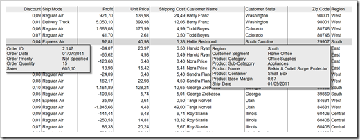
Today’s post provides such a feature to improve the navigation within wide data tables. Two additional textboxes automatically show the values of the invisible columns for the active row. No additional clicks necessary. Simply navigate through your worksheet and click on any cell in your data table and the textboxes will automatically update without obscuring the active row.

As usual, the article provides the Microsoft Excel workbook for free download.

The Challenge

I am sure you have encountered this situation many times before: you are working on a wide data table in Microsoft Excel with – let’s say – 30 or more columns. Even if you are using a very large monitor, it is likely that you do not see all columns of the table. However, when investigating data sets, you are also interested in values that are not visible at the moment. For instance, you see the customer name, the order date and the order quantity, but you do not see sales, the unit price, the discount and the shipping date.

What are you usually doing?

• Scrolling right and left again and again?
• Reorganizing the table to get the most important columns closer to each other?
• Freezing panes?
• Hiding and unhiding or – even better and easier to use – grouping columns and using the “+” and “-“ buttons to show and hide them?
• Opening a second window, arranging the windows tiled and switching back and forth?

Well, all this helps a bit, but it is still inconvenient and time-consuming, isn’t it?

There should be a feature which automatically shows you all values of all columns for the active row at a glance, without requiring any further clicks or actions.

The Idea

Some VBA could help. Probably the first idea that comes to your mind is a sub to display all values of the active row in a separate userform. Agreed, this is one step up, but there is an even better way: 

The recent article Tooltips on Microsoft Excel Tables showed how to use a shape textbox to display a tooltip for the active cell. Based on this approach we can also integrate 2 shape textboxes to show all values of the active row that are out of sight:

This way you can navigate through your table as you like and you will always see the entire data record of the active row at a glance. No need for scrolling back and forth anymore.

The Functionality

The VBA provided in the workbook (download link see below) automatically detects the active row and checks, which columns are visible on the screen. It highlights the active row with a grey fill color (this is optional) and shows the field headers and the values of the invisible columns vertically in one or 2 textboxes at the left and/or right of the active window. The shape textboxes are instantly updated as you move around in your worksheet by clicking into another cell or using the keyboard. If you click outside of the data table or if all columns are visible, the textboxes will automatically disappear.

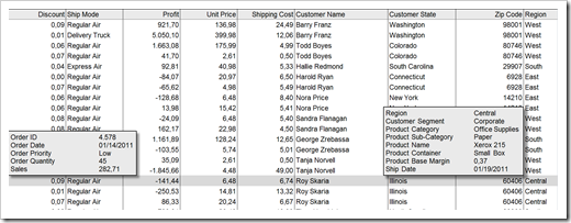
By default, the textboxes are located directly below the active row (see screenshot above). If the remaining real estate below the active row is not large enough to show the entire textboxes, the VBA automatically positions them above the active row as shown in this screenshot:

The Implementation

The implementation of this feature is very much along the lines of the code used to display the tooltips for the active cell described here: Tooltips on Microsoft Excel Tables.

These are the 2 most important things to know:

• Insert the code in the event procedure Worksheet_SelectionChange of the sheet module containing the data table. This way, the code will be executed every time the user selects another cell.
• The property ActiveWindow.VisibleRange: The name says it all. The property contains the ranged currently displayed on your screen. Thus, ActiveWindow.VisibleRange.Column is the first visible column and ActiveWindow.VisibleRange.Columns.Count is the number of visible columns. Based on this information you can easily calculate which columns are invisible and which headers and values have to be included in the shape textboxes

Here are the main steps of the VBA sub in pseudo code:

1. Update the cell with the active row on the worksheet (to trigger the Conditional Formatting of the active row)
2. Detect the relative row number in the data table
3. Detect the first and last visible column using ActiveWindow.VisibleRange and the numbers of invisible columns left and right of the visible range
4. Decide which textboxes have to be shown (if any) and make them visible or invisible
5. Exit the sub if the user clicked outside of the data table or if we do not have to show the textboxes
6. Define the ranges of the headers and the data
7. Concatenate the strings to be shown in the textboxes (separate the header from the values by a tab)
8. Assign the string to the text of the textboxes
9. Position the textboxes at the left and right of the active window either below the active row or (if not enough real estate left) above the active row

That’s it. Only 75 lines of VBA code (excluding empty lines and comments) and you are good to go. For more details on the implementation please refer to the Excel workbook provided for free download below.

The Excel 2003 version – a workaround

As already mentioned in an update to the article Tooltips on Microsoft Excel Tables, aligning headers and values using a tab in the VBA code does not work in Excel version 2003 and earlier. Excel shows ugly squared boxes (non printable characters) and the values are not aligned.

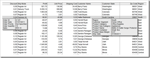
Here is a workaround for this issue: instead of using one string with tabs between headers and values, we are inserting additional textboxes. In other words, both extensions (left and right) consist of one textbox for the headers and one for the values, i.e. our worksheet has 4 textboxes in total:

The VBA code for this version is a bit different, but still pretty straight forward. If you are interested in the details, download the workbook (see below) and have a look.

Download

Here is the Microsoft Excel workbook for free download (2 textboxes and tabs in the texts to align the values), working well with Excel 2007/2010:

Download Display all Fields of a Row (Microsoft Excel 2007/2010, 52.2K)

If you are using Microsoft Excel 2003 or earlier, you will probably prefer the version with 4 textboxes instead of 2 to get around the tab issue described above:

Download Display all Fields of a Row version Excel 2003 (Microsoft Excel 2003, 120.5K)

How to use this in your own workbook

Here is a brief step-by-step how to transfer this feature to your own workbook (referring to the version with 2 textboxes):

1. Assign the range name “myData” to your table (including the headers of the columns).
2. Define a cell to store the number of the active row and call it “myActiveRow”
3. Add Conditional Formatting to highlight the active row based on the value of “myActiveRow”.
4. Insert 2 shape textboxes shapes, assign names to them (“myExtensionLeft” and “myExtensionRight”) and format them the way you like
5. Go to the VBE (ALT-F11) and paste the code from the workbook provided above into the sheet module of the worksheet containing the data table.

Steps 2 and 3 are optional. If you don’t want to have the actual row highlighted, simply skip these steps and delete the row in the VBA which is updating the cell with the active row. If you do not like the names I used, you can define your own, but you have to change the VBA accordingly.

That’s it.

Stay tuned.