A Microsoft Excel simulation model to reveal the revenue potential of billing increments in mobile or fixed-line tariffs
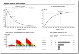 Be honest: do you know which incremental billing model is included in your mobile phone or fixed line tariff? No worries, I suppose most people do not know. However, incremental billing models represent a considerable part of mobile or fixed line operators’ revenues.
But what is incremental billing? It means that carriers are pricing calls in slices longer than a second. Full minute billing means – for instance – that you are paying two full minutes, although your call was only 61 seconds long.
How big is this effect of additional revenues? How much revenues do carriers make by using incremental billing?
Today’s post presents a simulation model to reveal and evaluate the revenue potential of different billing increment models. As always including the Microsoft Excel workbook for free download.
The background
What does incremental billing mean exactly? A billing increment is the smallest slice of a call a carrier will charge. Billing increment models usually have a nomenclature consisting of two numbers:
- Model 1/1 means a true per second billing: talk for 20 seconds, pay for 20 seconds.
- Model 60/1 means a minimum of 60 seconds and per second billing beyond the first minute. Talk for 20 seconds, pay for 60 seconds, talk for 61 seconds, pay for 61 seconds.
- Model 60/60 means full minute charging: talk for 20 seconds, pay for one minute, talk for 61 seconds, pay for two minutes and so forth.
These are the most common ones. However there are a variety of others (60/30, 10/10, 6/6, 18/6, etc.), working accordingly.
Let’s call a spade a spade. If you are having a tariff with a billing increment larger than one second, you will pay for air-time you never used. The effect of billing increments on the total amount of your phone bill depends not only on the incremental billing model, but also on the distribution of the call durations: the more short duration calls you have, the higher the impact and vice versa.
So, billing increments mean additional revenue potential for the carriers. But how large is this potential? How big are the additional revenues of different billing increments? A simulation model will help us to answer this question.
The probability of call durations
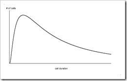 First and foremost, the additional revenue potential of a billing increment model depends on the call duration distribution, i.e. what is the probability of any given call duration?
For sure, this will be a positive or right skewed function as shown in the screenshot on the left. The mass of the distribution is concentrated on shorter call durations, e.g. a call lasting 3 minutes is more likely than a call lasting 30 minutes.
One function that reflects this is a log-normal distribution, i.e. a probability distribution of a variable whose logarithm is normally distributed. There are other options as well (like the Weibull distribution), but the log-normal distribution will do the job in our simulation model.
The implementation and the calculations
The simulation workbook consists of only two worksheets: the dashboard (see next section) and the calculation worksheet.
The used formulas on the sheet calculations are not too complex. There is one formula to create the log-normal probability function using the functions NORMDIST and LN. The formulas calculating the billable seconds per model use the functions QUOTIENT and MOD, but I think they are still pretty straight forward and easy to understand. To support the visualizations on the dashboard, there are some more calculations using MAX, MEDIAN, VLOOKUP, INDEX and MATCH, but still no rocket science. Everything else are simple basic arithmetical operations.
I am sure you will easily figure out how this works without further explanations.
For the sake of completeness: to limit the workbook to a reasonable size, the simulation is restricted to call durations up to 1,800 seconds, i.e. 30 minutes. Agreed a limitation, but no great effect on the results because of the right-skewness of the probability function.
The visualization
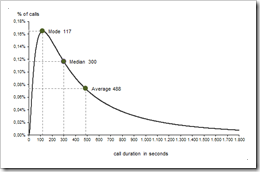 The probability function of the call duration is visualized using a standard XY scatter chart and 3 additional points to display the most important values at a glance:
the mode (the call duration that occurs most frequently), the median (50% of all calls are shorter, 50% are longer than the median) and the average call duration.
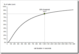 The distribution function shows the cumulative probabilities, i.e. the probability that a call is less or equal than a given call duration. The according chart (see left) visualizes how fast the probabilities converge to 100%. Again, this is an XY scatter chart and the additional point highlights and displays the threshold, where 80% of all calls are shorter or equal than this call duration.
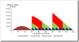 An area chart compares all billing increment models and visualizes the additional revenues compared to the model 1/1. This chart visualizes the way the models are working and at which call durations the most additional revenue is made.
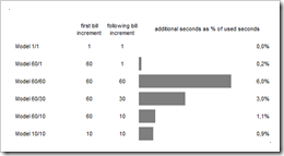 Finally, a very simple table and bar chart displays the most important results: how much additional revenue is made by each model compared to a billing per second (model 1/1). Furthermore, the user of the simulation workbook is able to define his own models by changing the values of the first and the following billing increments in seconds.
The simulation
The simulation part of the model focuses on the call duration probability function. By changing the mean and the standard deviation of the log-normal distribution (using the sliders), you may change the shape of the function and see immediately the impacts of your changes on the dashboard.
The workbook is restricted to 5 different billing increment models. However, you can easily change the predefined models by typing in new values for the first and the following bill increments in the cells M27:N31 on the dashboard. Thus you can adapt the simulation to your own requirements and what you consider to be reasonable.
The results
Here are two examples of simulation results:
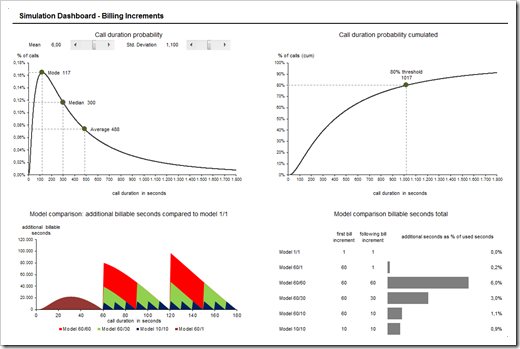
Let’s select a mean of the log-normal distribution of 6 and a standard deviation of 1.1. Most calls have a duration of 117 seconds, the median is 300 seconds and the average duration of a call is 488 seconds. A billing increment model 60/60 results in 6% higher revenues for the carrier than a model charging per seconds air-time (i.e. model 1/1). Not too bad, in my humble opinion.
If you choose a less right skewed distribution (mean: 6.4, standard deviation: 0.7), most calls last 363 seconds, the median is 411 seconds and the average call duration is 659 seconds (i.e. almost 11 minutes on average). The model 60/60 still produces 4.5% more revenues than a billing increment model 1/1.
Please be advised that both examples are arbitrarily chosen examples. I would assume they might represent reasonable probability functions. However, the parameters are made up, i.e. the given distribution is not based on real data of a real carrier.
The dashboard and the download link
Here is a larger screenshot of the one-page interactive simulation dashboard:
And here is the Microsoft Excel workbook for free download:
Download Simulation Billing Increment (Microsoft Excel 2003, zipped 425.8K)
What’s next?
Using mathematical functions in Microsoft Excel simulation and planning models are a very interesting topic. I am planning to write one more post on this during the next weeks. Furthermore I am having some more Tableau tips and workbooks in the pipeline.
Stay tuned.
Leave a Reply