Tag: microsoft excel

  • Interactive Bullet Graphs in Excel

    An interactive Multiple Row Bullet Graph in Excel displaying the gap and data labels only when hovering over a bar with the mouse

    The previous post presented An Alternative Design of Bullet Graphs in different versions and provided the implementation in a Microsoft Excel template workbook for free download.

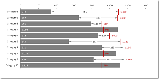
    Long time Clearly and Simply readers and contributors Matt Grams (check out Matt’s guest post: Bullet Graphs for Excel: A Simple Way?) and Leonid Koyfman (Leonid’s LinkedIn Profile) liked the alternative design in general, but also came up with a justified and constructive criticism regarding the Multiple Row Bullet Graph:

    Multiple Row Bullet Graph - click to enlargeThey noted that

    • the chart is too busy and a bit overloaded, especially if you are using it in a relatively small size, e.g. on a dashboard with other views
    • in certain edge cases, the data labels may overlap and become unreadable

    Valid points. I fully agree with Matt and Leonid.

    To make the chart less busy and more readable, Leonid suggested to turn it into an interactive Bullet Graph which displays the span of the gap (the thin line with arrows between actual bar and target line) and the data labels for gap and target only, if the user hovers over the bar with the mouse:
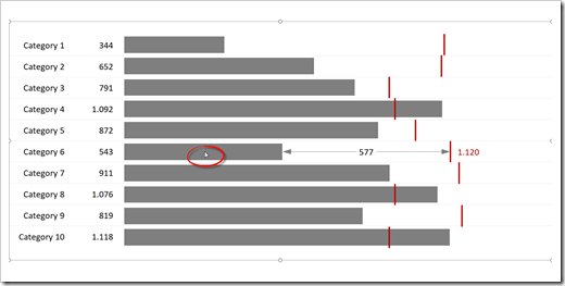
    Interactive Bullet Graph - click to enlargePlease note the mouse cursor over the bar of Category 6.

    The underlying technique and VBA code is described here: Mouse Driven Actions on Excel Dashboards.

    This interactive version definitely looks much cleaner, but it also comes with a few disadvantages:

    • The user has to activate the chart (click on the chart area) first to make the mouse hover action available
    • The approach is not applicable for dashboards delivered in a static version like PDF or printed. It only makes sense, if the user directly interacts with the chart in Excel
    • Unlike the original version, this solution requires VBA code
    • Because of the VBA code, it takes more time to transfer the template from the example workbook to your own model. You can’t simply drag the sheet over to your file, you also have to copy the entire code from all objects, modules and class modules
    • It requires Microsoft Excel 2013 or later

    Anyway, it still is a viable and interesting alternative to the original version.

    Here is the Excel 2013/2016 workbook for free download:

    Download Interactive Bullet Chart (zipped Microsoft Excel 2013-2016 workbook, 32K)

    Many thanks to Matt and Leonid for the feedback and suggestions. Much appreciated.

    Stay tuned.
  • An Alternative Design of Bullet Graphs

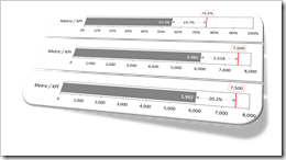
    An alternative design of Bullet Graphs: no qualitative ranges, additional data labels and a visualization of the performance gap (if applicable)

    Bullet Graph Alternative DesignMore than 10 years ago, Stephen Few of Perceptual Edge introduced the Bullet Graph: an alternative chart type to replace the formerly (and unfortunately sometimes still) popular gauges and speedometers on dashboards. A Bullet Graph visualizes a performance metric compared to a target (or other comparative measures) in a small, clear, simple and effective view. In the meantime, the Bullet Graph has become a widely respected, even standard chart type. Some major Data Visualization software applications like Tableau Software natively support Bullet Graphs.

    Back in 2009, Matt Grams described a possible solution of creating Bullet Graphs in Excel here on Clearly and Simply: Bullet Graphs for Excel: A Simple Way?

    I am using Bullet Graphs very often in my models for a very long time already, especially on Performance Measurement Reports and Dashboards. Starting with Stephen’s original design specification, I received a lot of feedback from my clients over the years. As a consequence, I made a few variations to the design of the Bullet Graph regarding the qualitative ranges, data labels and the performance gap (if applicable, i.e. if actual is smaller than target).

    Today’s article describes my variations of the original Bullet Graph design, explains the background why I made them, shows how to implement the charts in Microsoft Excel and provides the corresponding Excel workbook for free download.

    (more…)

  • User-defined Excel Chart Tooltips

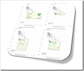
    How to provide different options of customized tooltips on a Microsoft Excel chart and let the user decide which one to display

    User Defined Tooltips in Microsoft ExcelOne of the previous posts described four different techniques how to create customizable, meaningful tooltips on XY Scatter Charts in Microsoft Excel:
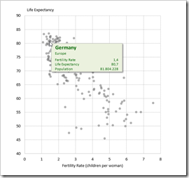
    Customizable Tooltips on Excel Charts

    Two of the approaches used a camera object (aka linked picture) to allow more formatting options of the tooltip.

    This idea can be taken one step further: with camera objects, you can easily provide more than one type of tooltip and let your user interactively select the tooltip which is most helpful for his analysis.

    Today’s article describes how to enable your user to select from five different tooltips with one single click: dimensions and measures, only a dimension and three additional charts displaying further information on the data point currently hovered over with the mouse. The post describes the idea and the implementation and of course makes the example workbooks available for free download.

    (more…)

  • Customizable Tooltips on Excel Charts

    How to create customizable, meaningful tooltips on XY Scatter Charts in Microsoft Excel

    Customizable Chart Tooltips on Excel XY Scatter ChartBack in December 2010, I published an article about Better Chart Tooltips with Microsoft Excel. The post described the weaknesses of Microsoft Excel’s standard chart tooltips and provided a VBA-based technique how to get to customizable, meaningful and more useful tooltips in Excel.
    Today, I would like to revisit this topic for several reasons:

    Firstly, Microsoft hasn’t done anything about this shortcoming in the versions 2013 and 2016. The problem of insufficient chart tooltips in Excel remains.

    Secondly, the workbook provided in 2010 implemented the better chart tooltips on another dashboard with additional features, which was published here: Bluffing Tableau Actions with Microsoft Excel. Many people have asked for a simplified, generic template only providing the tooltips on a standard XY Scatter chart.

    Next, reader Will Clark came up with the great idea of using a camera object instead of a simple textbox, in order to have more formatting options.

    Last, but not least, I discovered another approach for creating interactive charts in Excel. I already used and published this in several posts (Another Technique for Interactive Excel Charts, Selecting and Highlighting Areas on Excel Charts, Select Areas on a USA Map in Microsoft Excel and Zooming in and out of Excel Charts), but this technique is also viable for implementing chart tooltips.

    Today’s post will discuss again Excel’s shortcomings in terms of chart tooltips, briefly describe 4 different techniques how to overcome this issue and – as always – provide the Microsoft Excel workbooks for free download.

    (more…)

  • Select Areas on a USA Map in Microsoft Excel

    Interactive radial or rectangular area selection on a map of the United States in Microsoft Excel

    One of the recent posts demonstrated how to mimic Tableau’s rectangular and radial map selection features in Microsoft Excel:

    Selecting and Highlighting Areas on Excel Charts

    The example workbook used a map of Europe. Since more than 40% of my readership is located in the United States, I thought it might be a good idea to also share a template with a map of the USA. Here it is for free download:

    Download Select and Highlight Areas on a US Map (zipped Microsoft Excel 2010 – 2013 workbook, 1.3MB)

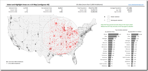
    This is an example screenshot of the dashboard:

    Interactive Selection on a USA Map in Excel - click to enlargeThe map (the contiguous 48 states, i.e. excluding Alaska and Hawaii) includes all cities in the United States with more than 5,000 inhabitants, divided into 2 categories (greater than or less than 500k inhabitants), visualized with different sizes of the dots.

    To define a radial or rectangular selection (choose with the radio buttons), keep the SHIFT key pressed, click somewhere on the map with the mouse key pressed, move the mouse to span the selection area and – as soon as you are done with your selection – release the mouse key. The metrics above the map and the bar charts (selection statistics by states) right to the map are updated on the fly.

    For more details on how to use the template and how this was implemented in Excel, please have a look at the original post.

    I hope this will be helpful, especially for my friends and readers in the United States.

    Stay tuned.