Artificial Intelligence in Microsoft Excel: watch a Neural Network solving a Travelling Salesman Problem
869 words, ~4 minutes read
 Terms like Artificial Intelligence, Machine Learning, Deep Learning and (Artificial) Neural Networks are all over the place nowadays.
If you are reading Tech News, Data Science blogs or your LinkedIn feed, it will be little short of a miracle, if you don’t see one of those expressions at least once.
This is just the revival of those techniques, though. Neural Networks, for one, have been around for many years. In the mid 1990s (!), I did some research and wrote my thesis about Artificial Neural Networks. We even had a blog post here on this topic 10 years ago: Where the rubber meets the road. For whatever reason, that article didn’t make many friends. I was always wondering why. Probably too academic and not visually appealing enough.
Now, with the recent revival of Artificial Intelligence and Neural Networks, I decided to give it another shot. Today’s post provides an updated, improved version of a Neural Network solving Travelling Salesman Problems in Microsoft Excel.
You always wanted to watch a Neural Network solving an optimization problem? If so, this article is for you. Either watch one of three videos provided in the post or download the Excel workbook and play around with it at your own speed. No add-in or third party software necessary. All you have to do is to enable macros.
The Algorithm
The Neural Network provided today is exactly the same as in the original post (Where the rubber meets the road). It is based on the article “an analogue approach to the travelling salesman problem using an elastic net method”, by Richard Durbin and David Willshaw published in Nature back in 1987.
Without going into the details of the mathematics, here is the basic idea of this approach:
Many other algorithms for solving TSPs start with one feasible solution and try to switch to better ones from iteration to iteration (i.e. shorter total tour length). The approach of Durbin and Willshaw is different: they don’t start with a feasible solution. They start with an elastic net (or adaptive ring), i.e. a circle of nodes where the number of nodes is a multiple of the number of cities of the TSP. This circle is gradually deformed until it finally passes through all cities and describes a feasible and short tour.
You can think of this ring as if it would be a rubber band. In each iteration, the Neural Network randomly selects a city, finds the nearest node on the ring and pulls the node and its neighbours towards this city. If you visualize this behaviour of the algorithm, it looks as if this rubber band is deformed and elongated until a feasible solution is found. The tension of the rubber band guarantees that dragging the rubber band complies with the objective function of the TSP, i.e. to minimize the total tour length.
The Updated Version
As already stated above, the used algorithm is exactly the same as in the original post. However, I made quite a few changes in the workbook to make the handling of the model easier and the views more interesting:
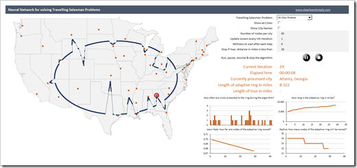
 The most obvious change is the map. Instead of showing generic points in the Euclidean space, today’s workbook solves Travelling Salesman Problems through cities of the United States and provides the geospatial context with a US map in the background.
Furthermore, I simplified the dashboard:
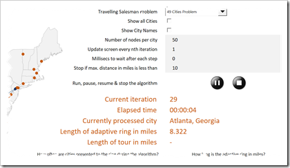
 Only the most important user-selections are still available on the dashboard and only a selection of results is shown.
With that said, I did not only simplify, I also added a few helpful features:
- With the play buttons, you can start, pause, resume and stop the algorithm at any time
- With the two checkboxes, you can decide whether or not all cities of the US shall be shown on the map (i.e. not only the ones of the TSP) and whether or not the names of the TSP cities shall be displayed
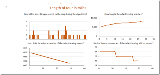
At the bottom right of the dashboard, four charts visualize some key metrics of the algorithm during execution:
- a column chart shows the distribution of the cities, i.e. how often the cities are randomly selected and processed during the algorithm
- the three line charts visualize the development of the length of the adaptive ring, the decreasing learn rate and the size of the radius, i.e. the decreasing number of nodes being moved on the ring
Now, let’s see this in action:
Watch examples right here in a video…
Here is a 10 cities TSP. The algorithm is slowed down intentionally by waiting 200 milliseconds after each step to better understand how the Neural Network works:
The next video shows how a 20 cities TSP is solved. No waiting time, but still updating the screen after each iteration:
Finally, a 100 cities TSP. The views on the dashboard are updated every 50th iteration:
… or download the workbook and have a look for yourself
Not only interested in watching the videos, but also in playing around with the model or even dissecting the code? Here you go:
Download Neural Network Solving TSP (zipped Excel workbook, 663K)
Stay tuned.

Leave a Reply