How to create a Summary Table in Power Query with aggregated values of the original data source without importing the entire data into Excel
A frequent use case of Power Query (aka Get and Transform) is to connect to an external, big data source, filter and remove data in a query and load only a fraction of all rows into the Excel workbook.
This will ensure you only carry along the parts of the data in your workbook you really need and will thereby keep the size lean and the performance fast.
Although you do not need the original data on row level in your workbook, you might be interested in a couple of aggregated measures of the original data table, e.g. the total sum of a column, the count of rows, the distinct count of entries (unique values) in a column, etc.
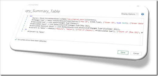
Today’s post explains how to create a Summary Table with defined aggregations on the original data without loading the entire source. The key of the solution is the M-function #table.
As always, the post comes with an example workbook for free download.
What for?
Why would you need a summary table in the first place? Well, according to my experiences, there are 2 main use cases for this:
- You need the aggregated values from the original table for putting your data into context by calculating measures relative to the unfiltered data, e.g. the percentage of total sales or the count of filtered orders compared to the total count of orders
- If your workbook will undergo a review by internal or public auditors, you may have to provide defined measures of the original data in order to allow checks if the correct and entire source data has been used
There are certainly many more uses cases, but these two are the ones I am facing in almost all of my projects.
The Example
For explaining the technique I will use a very simple data set. The original data is a table of orders taken from Tableau’s Sample Superstore. A query imports the data and filters it by [City] = “Los Angeles”. This reduces the count of rows from 9,994 to 747.
The request is now to also have the following measures of the source data available in the Excel workbook:
- The total sum of [Sales]
- The count of [Row ID]
- The distinct count of [Customer ID], i.e. the count of unique customers
How to create a Summary Table with Power Query: a step-by-step tutorial
Step 1: Connect to the Original Data
First, you create a new query and connect to the external source data. You know how to do that, don’t you?
In most cases, Power Query automatically promotes the headers and changes the types. You get to something like this:
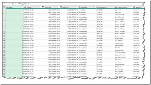 If this is not the case for your data, promoting headers and changing data types in Power Query are standard features available on the Transform tab and should be a walk in the park.
Step 2: Create the first aggregation – Sum of [Sales]
Select the column [Sales], go to the Transform tab of the ribbon, click on Statistics and Sum:
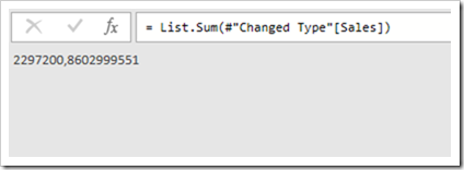
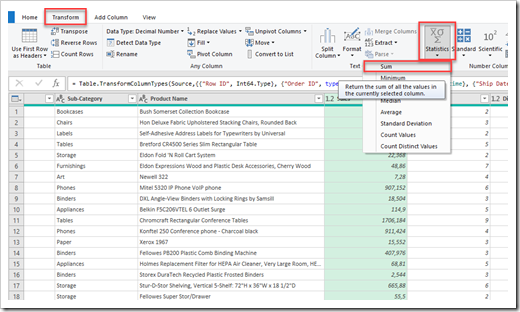 As a result the table is gone and only the total sum of [Sales] is displayed:
 Step 3: Create another aggregation
We have the sum of [Sales] now, but we also want the count of [Row ID] and the distinct count of [Customer ID].
Directly after the step of calculating the sum of [Sales], the Statistics command is not available anymore. This is reasonable, because aggregations like sum or average do not make sense for a single number.
So, how do we get around that? Well, as always, there is more than one way to skin the cat. Here are three possible options:
Option 3a: Link back to the last step which resulted in a table
In the Applied Steps pane, right click on the last step (Calculated Sum) and select Insert Step After:
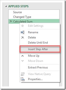 Power Query inserts a new step, calls it Custom1 and automatically sets it as a reference to the previous step Calculated Sum:
 Now, go to the formula bar of the Power Query Editor and replace “Calculated Sum” by “Changed Type”. Thereby the new step refers to the step “Changed Type” and produces the same result, i.e. the table shown in step 2.
Next, select the column [Row ID], go to the Transform tab, click on Statistics and Count, just like we did for the sum in step 2.
Option 3b: Insert a new step after “Changed Type”
Alternatively, you can select the step “Changed Type” in the Applied Steps pane, select the column [Row ID] and insert the calculation of the count similar to the way we inserted the sum (Transform|Statistics|Count).
Although this looks good at first sight, we are not done yet. If you now click on the step “Calculated Sum”, you will see this:
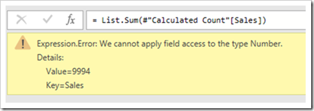 What is the problem here? Since we inserted the new step to calculate the count between the steps “Changed Type” and “Calculated Sum”, Power Query changed the reference of the calculated sum formula to the previous step, i.e. to “Calculated Count”. And performing the sum requires the column [Sales], but this isn’t there anymore.
How to fix that? Simply go to the formula bar and replace “Calculated Count” by “Changed Type” and the error disappears:
 Option 3c: Insert a step at the end and manually type in the M-code
The last option is definitely for the more advanced users of Power Query, who are familiar with M code and its syntax. But it is certainly the fastest and most elegant way.
Insert a step at the end just like in option 3a, go to the formula bar and replace what is there by the M-statement to calculate the count:
= List.NonNullCount(#”Changed Type”[Row ID])
Please note that the function call List.NonNullCount refers to the column [Row ID] of the step “Changed Type”.
Step 4: Create further aggregations
For further aggregations like Distinct Count, Averages or Sums of other columns, etc. simply repeat step 3 for each of them, select the according column and use the desired aggregation function from the statistics menu.
Step 5: Create the table
We now have calculated all the aggregations of the original data we want to load into our workbook. The last step of the query, however, results in a single number. If we would load that, only the final aggregation would be loaded into an Excel table.
Please be advised that all other steps (calculated sum and count) are still available. All we have to do now is to combine these results in one table.
The M-function #table is what we need and here is its syntax:
#table (columns as any, rows as any) as any
Please have a look at the M Reference – #table for the details.
This is how the #table function looks like in our example:
= #table({“Measure”, “Value”},
{
{“Sum of [Sales]”, #”Calculated Sum”},
{“Count of [Row ID]”, #”Calculated Count”},
{“Distinct Count of [Customer ID]”, #”Calculated Distinct Count”}
})
With {“Measure”, “Value”} as the first parameter passed to the function, we define our table to have 2 columns with the specified column names.
{“Sum of [Sales]”, #”Calculated Sum”} creates the first row of the data range of the table: the text “Sum of [Sales]” will go to the first column and the result of our applied step #”Calculated Sum” will go into the second column.
{“Count of [Row ID]”, #”Calculated Count”} inserts a second row in our table with “Count of [Row ID]” in the first column and the result of #”Calculated Count” in the second. And so forth.
Now, all you have to do is to insert a new step at the end of the query and type the statement above into the formula bar. If you copy the statement from the text above, please remove the line feeds before you paste it into the formula bar.
And that’s it.
Here is our Power Query Summary Table:
 We can now load this into Excel’s data model and/or to an Excel table.
Download
Here is the example workbook used to produce the screenshots above for free download:
Download Summary Table with Power Query (zipped Microsoft Excel workbook, 1.4MB)
Please be advised that this workbook includes the original, unfiltered data in a table which is then used as the data source for the queries.
It goes without saying that you don’t need a summary table if you have the source data inside the workbook. I included the original data only to facilitate the download and usage of the example workbook. Just imagine the source data of the queries would not be a table inside the workbook, but an external CSV or Excel file or a table in a database. In this scenario, a Summary Table will definitely make sense.
Please let me know what you think.
Stay tuned.
Leave a Reply