Different techniques of how to color encode data points of a bar chart based on a second data series in Microsoft Excel
 Color encoding can be a very powerful technique for data visualization. Heat Maps or Choropleth Maps are classical examples of visualizing data by color encoding.
However, you can add color encoding to almost any kind of visualization. For instance, using colors on bar charts can display additional information of the data and – if used carefully – considerably improve the significance of the visualization without requiring further real estate on a dashboard.
With Tableau Software, color encoding your charts is a piece of cake. Simply drag the dimension or measure to the color shelf and you are done. Microsoft Excel has no comparable built-in functionality. However, this doesn’t mean you can’t use color encoding in your Excel charts. Of course you can.
Today’s post describes different techniques of how to color encode Microsoft Excel bar charts, with or without using VBA. As usual, all described techniques are coming with an example workbook for free download.
The Basic Idea
The basic idea is simple and obvious: Add another dimension or measure to your bar chart by coloring the bars according to the values of another data series.
One practical example would be a bar chart displaying one performance KPI of sales agents (e.g. sales figures, revenues, or the like) using the lengths of the bars and visualizing their sales regions (e.g. north, east, south, west) by coloring the bars with four different colors. More information in the same amount of real estate on your dashboard.
Microsoft Excel does not provide a built-in feature to do this color encoding, but – of course – this does not mean you can’t do it at all. As always, there is more than one way to skin the cat. Here are three different ways of how to accomplish this with Microsoft Excel.
Technique 1 – Several Data Series
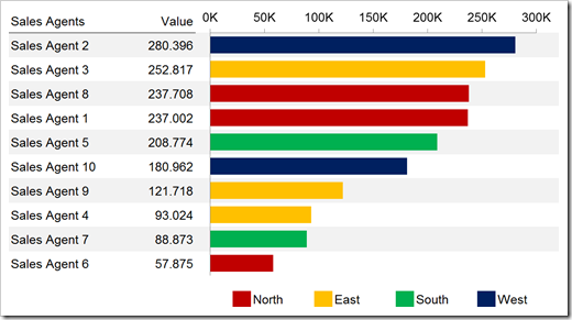
I am sure you know this technique already. If you want to color encode categories (like in the example mentioned above), you add as many data series to your bar chart as you need (e.g. four sales regions in our example above) and format them using different fill colors.
A very simple IF-formula makes sure each data series contains the KPI values only if the row (i.e. the sales agent) belongs to the according category (i.e. the sales region) and NV() otherwise.
The result could look like this:
Here is an example workbook for free download:
Download Colored Bar Chart Data Series (Categories) – (Excel 2003 workbook, 79K)
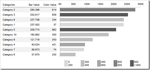
You can use exactly the same technique if you want to color code a measure instead of a dimension. All you have to do is to cluster the values in categories, e.g. by defining value ranges or using percentiles.
You would probably use different hues of the same color instead of different colors, like this:
Here is the according workbook for free download:
Download Colored Bar Chart Data Series (Measures) – (Excel 2003 workbook, 86.5K)
Technique 2 – Change the Fill Color using VBA
You don’t mind using some simple VBA routines in your workbook? Good. A very small VBA sub can automatically change the fill color of the bars. Thus, you need only one data series in your bar chart. The set-up is very similar to technique 1 (color encoding a measure):
- Define value ranges (as many as you like)
- Define the color scale using the fill color of cells
- Use a simple MATCH formula to assign each value to the correct value range
- The rest is done by a very simple VBA routine looping through all data points in a For Next statement and setting the fill color to the according fill color of the range this value belongs to.
Have a look at the worksheet [calculation] and the small VBA routine of this workbook:
Download Colored Bar Chart Fill Color (VBA) – (Excel 2003 workbook, 89K)
The VBA sub “ColorBarChart” is assigned to the spinner on the dashboard, i.e. the coloring changes each time you are switching to another data set. Of course, you could also call this sub from a Worksheet_Calculate or any other event driven procedure.
Technique 3 – Change the Transparencies using VBA
This technique is limited to Excel 2007 or later. Like technique 2, it uses VBA. However, it does not change the fill color of the bars, but the transparencies. The set-up of the workbook is easier than with the other 2 techniques. Like technique 2, you need only one data series in your bar chart. You do not have to define range values, all you have to do is to create a helper column calculating the transparency values with a pretty simply formula.
Here is an example how this would look like:
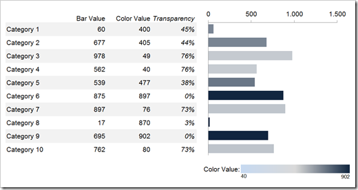
The VBA procedure is very similar to the one used for technique 2. Instead of changing the property .Interior.ColorIndex, it changes .Fill.Format.Transparency, using the percentage values in the helper column (see above).
That’s it. One helper column and 8 lines of VBA code and you are good to go.
Here is the workbook for free download:
Download Colored Bar Chart Transparencies (VBA) – (Excel 2007 workbook, 28.8K)
Please use this with caution
Color coding is a very interesting way of visualizing data, no doubt about it. However, you should always think twice before using it. From my point of view, color coding sales regions of agents (as shown in the example for technique 1) adds a lot of very useful information. Imagine the bar chart would include more than 10 agents. You could easily see from the colors of the bar that e.g. 5 out of 10 of the top performers are coming from one sales region.
However, human eyes respectively the human brain are not very good in comparing values by color hues. For instance I would not recommend using a bar chart displaying the revenues of your company branches as the bars and their profits as the color. I would use 2 aligned bar charts instead. This makes both KPIs comparable at a glance.
Still, I do believe there are some use cases where coloring bars can be a viable alternative. All you have to do is to thoroughly think about which visualization tells your story best.
A Practical Example – A Color Coded Tornado Chart
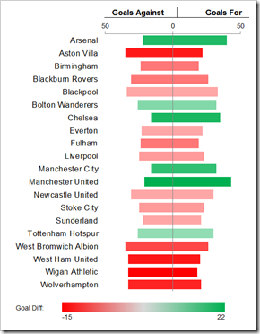 The recent post described my “non-entry” to the The Tableau Interactive Sports "Viz" Contest: The History of Premier League Statistics.
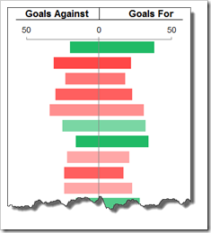
This Tableau workbook included a variety of tables and visualizations and one of them used color coded bar charts: Dashboard 2 contained a chart showing the goals of each team at any point in time: Goals for, goals against and goal difference.
A tornado chart is not far to seek for this data set. One bar for each team, goals for on the right of the vertical axis and goals against on the left. This is pretty intuitive, I think.
But what about the goal difference? Sure, the bars leaning to the right are the ones with the better goal difference and vice versa. However, have a look at the example shown above. Imagine you would not have the color coding, would you be able to see at a glance that Aston Villa’s goal difference is worse than the one of Blackburn Rovers or that Liverpool’s goal difference is negative? I do not think so.
Thus, from my point of view this is a very good example of how to effectively use color coding on a bar or tornado chart. Sure, you can always add another bar chart displaying the goal differences, but if you are short of real estate on your dashboard, color coding can be a viable alternative in this case.
The implementation isn’t too difficult. It somehow is a combination of technique 1 and 3: four data series in the chart and a slightly changed VBA routine adjusting the transparencies of all 4 data series. Nothing new under the sun. Here is the example workbook for free download:
Download Colored Tornado Chart – (Excel 2007 workbook, 60.1K)
Acknowledgements
Many thanks go again to my friend Dan L, who was once more kind enough to invest some of his precious time reviewing my ideas and workbooks. A big time thank you very much, Dan. Your feedback is invaluable.
What’s next?
I am planning to have two Tableau articles during the next weeks: a new Tableau Quick Tip and an article on the making of the Premier League Historical Statistics.
If you are more interested in articles on Microsoft Excel, please hang in there. I am also working on a follow-up post to the Pivot Table with texts in the value area and on an article about how to drill-down within an Excel dashboard.
Stay tuned.
Leave a Reply