Tooltips on Microsoft Excel Tables

How to display Tooltips on Microsoft Excel Tables including additional information on the selected cell and aggregation results for the entire column
Microsoft Excel Table TooltipsTooltips are a very helpful feature when exploring and investigating data. On charts and on plain data tables. When referring to tooltips, I am talking about additional details on the data currently selected or hovered over using the mouse. Tooltips could include other dimensions and measures, calculations or aggregated information like totals or averages.

Tableau Software provides very powerful and easy to use tooltips. If you are working with Tableau, I once again recommend having a look at Andy Cotgreave’s great Tableau tooltip articles on the Data Studio (Tableau Tooltips: Conditional Formatting or Charts inside a tooltip? Yes, we can.). Thanks again for sharing, Andy.

Compared to Tableau, Microsoft Excel’s tooltips functionality is next to nothing. We already had a post showing how to improve tooltips on Excel charts: Better Chart Tooltips with Microsoft Excel 2010.

However, tooltips can be very helpful in plain data tables as well. Sure, Excel automatically displays some calculated aggregations of the selected range in the status bar. Yet, this is not enough. Your eyes always have to jump down to the status bar to see the information, the displayed quick calculations are limited and inflexible and you always have to select the range first. If you are working with larger data tables, you may wish for tooltips providing additional information on the selected value (like the percentage of total, the rank, etc.) and on aggregations across the entire column (like sum, average, etc.).

Today’s post provides two slightly different approaches how to create better tooltips on Microsoft Excel tables. As usual including the Excel workbooks for free download.

The Challenge

You are certainly aware of the fact that Excel automatically shows some information on the aggregation of the currently selected cells in the status bar:

Quick Calculations Microsoft Excel Status Bar  - click to enlarge
In Excel versions prior to 2007, the status bar was limited to one calculation, but you could still switch from the default sum to something else. Since 2007, you are able to show several calculations simultaneously. This is a very helpful feature for ad-hoc data analysis. Comparable to Tableau’s Summary Card.

However, it is designed to show the quick calculations for the currently selected cell range. If you are working in larger data tables, you are probably interested in aggregations of the entire active column without being forced to select the column first. Sure, you can add additional cells including the aggregation formulas e.g. above the data table and I guess this is what most people do.

Yet, if you are short of real estate on your worksheet (a dashboard, for instance) or if you want to add additional information on the active cell (like the percentage of total), a tooltip can be a viable alternative:

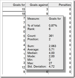
As soon as you click on any cell within the data table (excluding the headers), a tooltip appears with additional information on the selected cell (% of total, rank within all data entries of this column, etc.) and aggregated measures of the entire column (sum, average, minimum, maximum, etc.):
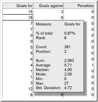
Tooltip Numeric Column - click to enlargeIf you select a column with non-numeric data, a different tooltip is displayed:
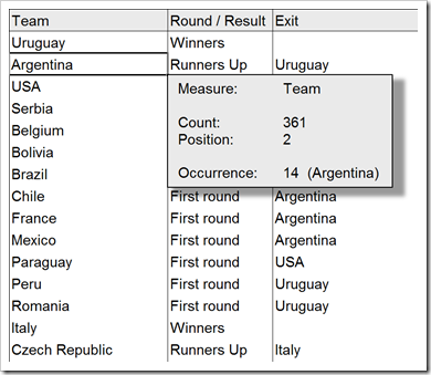
Tooltip Text Column - click to enlargeAs soon as you click outside of the data table, the tooltip automatically disappears.

Basics of the Implementation

The basic idea is as simple as can be: add a textbox to the worksheet and use VBA to

  • show the textbox if the active cell is within the data table and hide it otherwise
  • position the textbox at the bottom right of the active cell
  • calculate some additional information on the active cell and some aggregations for the entire column and display it in the textbox

Approach 1 – VBA only

The approach does almost everything in the VBA code. All you need in the worksheet itself is the data, a name for the data range (e.g. “myDashboardTable”) and a text box with a name (e.g. “myShpTooltip”).

The VBA code will then show or hide the tooltip, relocate it, do the calculations and show the results in the textbox. Here are the main steps of the VBA:

  • Check if the active cell is within the data table. If not, hide the textbox and exit the sub

Otherwise

  • Define the range of the active column
  • Check if the active column contains numbers or alphanumerical data
  • Calculate aggregation values based on the result of the previous check (numbers or text values)
  • Create a string to be shown in the tooltip
  • Assign this string to the textbox
  • Relocate the textbox to the bottom right of the active cell
  • Resize the textbox
  • Show the textbox

This procedure is defined in the event sub “Worksheet_SelectionChange” of the worksheet containing the data. This way, the tooltip is updated (or hidden) every time the user selects another cell (with the mouse or the keyboard).

Approach 2 – VBA and Worksheet Calculations

Approach 2 uses the same basic principle and VBA procedure. However, the content of the textbox is not created using VBA. Instead, there is a second worksheet called [calculations]. The VBA updates 2 cells with the row and the column of the active cell. The aggregations and other calculations are then conducted by formulas on the worksheet and the VBA simply refers to the results of those formula cells to create the string displayed in the tooltip.

The advantage of this approach is the fact that changing the content of the tooltip is much more convenient, since you only have to change the cells on sheet [calculation] instead of being forced to adapt the VBA. The disadvantage of approach 2 is the additional worksheet and more named formulas. From my point of view, it is easier to implement and easier to maintain. Thus, I would recommend using approach 2.

Both approaches require only relatively small VBA routines: 61 respectively 54 lines of code (excluding empty lines and comments). No big deal. If you are interested in the details, download the workbooks and have a look. The workbooks provided below are without any protection.

The Performance

I implemented and tested the VBA code using an extract of an example data set of the FIFA World Cup results (1930 to 2006), which I already used for a Tableau post here: FIFA World Cup Statistics with Tableau. With this limited set of data (361 data rows), the performance of the tooltips is very good.

If you are using a larger data base (I also tested it with a database of 65,500 rows), the performance of the tooltips in text columns is still acceptable. The numeric columns are a different story. Doing all the recalculations required for the columns with numerical data takes a few seconds. Check it out and decide for yourself. If the performance is too slow for your data, you could still delete some of the calculations shown in the tooltip.

The Download Links

Here is the Microsoft Excel workbook of approach 1 (VBA only) for free download:

Download Excel Table Tooltips VBA only (Microsoft Excel 2003, 93K)

And here is the workbook using approach 2 (VBA and worksheet calculations):

Download Excel Table Tooltips Worksheet and VBA (Microsoft Excel 2003, 100.5K)

Enjoy…

…and stay tuned.

Update on Friday, May 06, 2011

I just noticed one weakness in the workbook provided above, if you are using Microsoft Excel 2003 or earlier. The implementation works in general, however, the tabs inserted by the VBA code (vbTab) to nicely align the values are not working in Excel versions prior to 2007. Instead, you see an ugly squared box (representing a non-printable character) and the headers and the values are not aligned.

Thus, I implemented a different approach to make the table tooltips look nice in Excel 2003, too. To get there, I am using 2 textboxes, one with the headers and one with the values. Some more VBA required, but still pretty straight forward. Have a look:

Download Excel Table Tooltips Worksheet and VBA 2003 (Microsoft Excel 2003, 119K)

Comments

20 responses to “Tooltips on Microsoft Excel Tables”

  1. SteveT Avatar
    SteveT

    Great Idea. I guess if you have real estate on the dashboard you could use check boxes and show the data on the selected item. This would allow a 3rd option of NO VBA and just Worksheet calculations.

  2. Robert Avatar

    Steve,
    many thanks for your comment. I agree, your idea is a possible way of implementing this without VBA.
    However, using VBA has some considerable advantages:
    Firstly, you are not restricted to a relatively small number of rows. Sure, on dashboards your data tables will probably have no more than let’s say 10 or 20 rows and inserting 20 check boxes is still acceptable. Yet, using VBA allows you to implement this on a very large data table even if you have a couple of thousand rows. You wouldn’t want to insert thousand check boxes, would you?
    Secondly, the VBA automatically positions the text box to the bottom right of the active cell. Without VBA, you have to use a static part of the sheet and your eyes have to jump up or down to see the details.
    I like your idea, but I still prefer the VBA solution. Anyway, thanks for the idea. Greatly appreciated.

  3. Mich Avatar
    Mich

    Hi,
    This is a great post, very informative. I have been experimenting with the code, trying to expand the textbox to include several columns of information, however I cannot get the formatting quite right. I would like the result to look more like a table but it does not turn out that way. The vbtab spacing is not uniform for each row of data. Any advice on how format the ranges so the result looks tabular.

  4. Robert Avatar

    Mich,
    thanks for your comment. I just checked and added additional “columns” to the tooltip, separated by vbTab and it worked like a charm (using Excel 2010).
    Which version of Excel are you using? If you are using Excel 2003 or earlier, the vbTab is not working.
    Did you notice the update at the end of the article? It provides another approach using one textbox for each column of the tooltip. Needs more textboxes, but works well with Excel 2003.

  5. Mich Avatar
    Mich

    Robert,
    Thank you for the response. I did see the update but I wanted to see how flexible the first solution could be. I think the issue surrounds my attempt to input text instead of numbers after each vtab. I am finding that the length of the tab shown after each entry on the textbox seems to be dependent on the length of the text it precedes. Thus the final output does not look tabular at all as the columns are not aligned. I am using Excel 2007. I will try the second solution but I suspect the aesthetics may suffer due to the nature of the info I am trying to display.
    Thanks again
    Mich

  6. Robert Avatar

    Mich,
    you are welcome. I understand. If you are using texts and the entries in one column vary considerably in length, you could use several vbTabs between the columns (as many as necessary to align the columns nicely). But this is probably not a reasonable way of doing this.
    Another idea would be using a camera object instead of a textbox. This way you could define the table including the different columns somewhere in the workbook and link the camera to this range. Concatenating the string in the VBA code wouldn’t be necessary anymore. The VBA would only hide and unhide the camera and position it correctly at the bottom right of the active cell. Let me know if you need further information on how to do this.

  7. mich Avatar
    mich

    Hi Robert,
    Thanks again you have been very helpful. That solution sounds very intuitive I will try it and let you know. I did follow your initial advice to use multiple textboxes and it worked like a charm. I had to do some formatting to make it look like one seamless textbox but it was exactly what I had envisioned.
    Mich

  8. Ulrik Avatar
    Ulrik

    Great post with some excellent ideas!
    I don’t know how you find the time for making all these excellent posts – but thank you, and please keep up the good work!
    I have been experimenting quite a bit with this workbook as well as the one with the chart tooltips – sort of comibining the two. And I am happy to say it works really well!
    One thing that I am missing though, is that it would be great if there was a way to format the text strings (bold, color, underline, font size, etc.) in the VBA Code. I am aware that I could set up a table and format it as I wished and then use a camera object, but I generally find the picture quality of the camera wanting.
    Ulrik

  9. Mich Avatar
    Mich

    Hi Robert,
    I have a question for you. Is it possible to change the color of the textbox or make the color conditional on some value in the spreadsheet? I have been experimenting with a couple of commands (i.e. textbox.backcolor = vbGreen) but nothing seem to work.
    Thanks for you help
    Mich

  10. Robert Avatar

    Mich,
    the following line of code changes the fill color of the textbox to red:
    Worksheets(1).Shapes(“myshpTooltip”).Fill.ForeColor.RGB = RGB(255, 0, 0)
    I hope this will be helpful.

  11. mich Avatar
    mich

    Hi Robert,
    Many thanks, it worked perfectly
    Mich

  12. Jonesybj Avatar
    Jonesybj

    Hi, stumbled accross this while looking to make tooltips for a spreadsheet i’m working on for gear enchants and mods for Star Wars the Old Republic game. basically choose a mod from a data validation click on cell to bring up tooltip with values. is there a way to not be able to click on the Text Box?? i selected not edit objects in the protect sheet but when doing this nothing updates in the text box. this is coming at end user point of view.
    Cheers
    Brent

  13. Robert Avatar

    Brent,
    protecting the worksheet with an unchecked “Edit Objects” option is the right direction. However, you have to unprotect the worksheet in the VBA before you update the text and protect it again afterwards, like this:
    ActiveSheet.Unprotect
    .TextFrame.Characters.Text = strToolTipText
    ActiveSheet.Protect

  14. Jonesybj Avatar
    Jonesybj

    sweet thanks
    Brent

  15. Arul Avatar
    Arul

    Nice Idea
    Instead of a text box, which is adding a new shape(textbox) Excel has a built in functionality which allows users to show tool tips on cell selection. In the data validataion there is a tab called input message. Using this you can show tool tips. We just create our string and place it in the code below. we don’t set any validation rules on the cells, just the input message. Because it is non editable and gives the user no hint of what that shape is, it looks more professional. but then that’s just my opinion.
    With Mycell.Validation
    .InputTitle = “The title you make here”
    .InputMessage = “The string you create here”
    End With

  16. Arul Avatar
    Arul

    In fact you can avoid the slight lag by creating the string inside an excel cell itself by using char(10) for the carriage return. and iferror or if(iserror) combinations to omit out cells that evaluate to an error.
    Thanks,
    Arul

  17. Robert Avatar

    Arul,
    thanks for your comment. The data validation input message is an interesting idea and alternative to the textbox technique. However I would still prefer the textbox for 2 reasons:
    1. As far as I know, there is no way to format the data validation input message, like the fill color, font type and size, etc. The textbox provides all formatting options of a shape and is – in this respect – more flexible than the input message.
    2. There is a small annoyance coming with the input message: if the user clicks on the message and drags it somewhere else, the input message will stay at this position, even if you change the selected cell. The position of the input message will only be re-initialized and move with the selected cell again after you closed and reopened the workbook. In the textbox technique, the VBA takes care of the correct position of the textbox, so you do not have this somehow strange behavior.
    Anyway, I agree with you: the input message is easier to set up (VBA code is way simpler). So, if you are fine with the default formatting and do not care about the described annoyance above, the input message is a viable alternative.
    Thanks for sharing this idea.

  18. Mauk Avatar
    Mauk

    Great post! Although first link ( Download Excel Table Tooltips VBA only (Microsoft Excel 2003, 93K) ) returns error: An error occurred. Please wait a few minutes and try your request again.

  19. Robert Avatar

    Mauk,
    thanks for letting me know. I fixed the link, please try again.

  20. Mauk Avatar
    Mauk

    Very nice, thank you!

Leave a Reply

Your email address will not be published. Required fields are marked *