Scroll and Search in Excel Dashboard Tables

How to add a search bar and search functionality to a scrollable table on a Microsoft Excel Dashboard
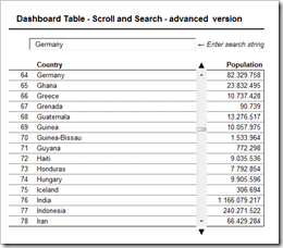
Scroll and Search in Excel Dashboard Tables - click to enlargeMore than 2 years back my friend and Microsoft Excel MVP Chandoo gave me the opportunity to publish a series of 6 articles on how to implement interactive Microsoft Excel dashboards on his excellent blog Chandoo.org: KPI dashboards with Microsoft Excel. To my surprise these articles still seem to be very popular over at Chandoo.org and Chandoo’s readers even keep on commenting these posts.

Yesterday Milind raised an interesting question: Is it possible to add a search bar to the dashboard to look up values in the source data and automatically scroll up or down to the according row of the search result?

Although Hui already explained how to do this in a comment, I decided to elaborate a little bit on the possible options in this additional article here on Clearly and Simply. Today’s post describes 2 different techniques on how to add a search functionality to a dashboard with a scrollable data table. As always, including the Microsoft Excel workbooks for free download.

The challenge

The original post KPI dashboards with Microsoft Excel described a very simply, yet effective technique to show an extract of a larger data table on an interactive dashboard using a form control scrollbar and OFFSET formulas. If it is a very large database, a search functionality can be a very useful additional interactive feature: it enables the user to immediately jump to a certain part in the data table without being forced to scroll up and down.

Option 1 – Use a cell to enter the search string

Here is the obvious idea: define a cell as the search string input field, use a MATCH formula to find the entered search string in the raw data and add some lines of VBA to overwrite the target cell of the scroll bar with the result of the MATCH formula. Here is the step-by-step description of what to change in the original workbook:

  1. Add a cell to your dashboard: the input field for the search string
  2. Assign a name to this cell (“mySearchString”)
  3. Use a new cell on the worksheet “Control” and type in the following formula:

    =IF(ISNA(MATCH(mySearchString,Data!$C$5:$C$194,1)),1,
    MATCH(mySearchString,Data!$C$5:$C$194,1)+
    IF (ISNA(MATCH(mySearchString,Data!$C$5:$C$194,0)),1,0))

    Here is this formula in pseudo code:

    If {neither the exact string nor a value less than this string can be found} Then
        {1}
    Else
        {position of the largest value less or equal than the search string}
        IF {the exact string can not be found} Then {add 1}
    End If

    The formula returns 1 if nothing similar to the search string can be found, the position of the search string, if an exact match can be found and it adds 1 to the position of the closest match, if the exact string couldn’t be found.

  4. Define another new cell on the worksheet “Control”, assign a name (“myOverwritePosition”) and type in an MIN formula to prevent the overwrite position from becoming larger than the defined maximum start position.
  5. Add the following Sub to the code of your worksheet “Dashboard”:

    Private Sub Worksheet_Change(ByVal Target As Range)
        If Target.Address = Range("mySearchString").Address Then Call UpdateValues
    End Sub

  6. Finally insert a new VBA module and copy the following Sub to it:

    Sub UpdateValues()
        Range("myStartPosition").Value = Range("myOverwritePosition").Value
    End Sub

That’s it. A couple of additional cells, 2 formulas and 2 small VBA Subs. Here is the workbook for free download:

Download Dashboard Table Scroll and Search simple v01 (Microsoft Excel 2003, 141.5K)

Option 2 – Use an ActiveX textbox to enter the search string

A slightly different approach, but only a few changes are needed:

  1. Insert an ActiveX text box on the dashboard
  2. Add another cell to the Control worksheet and assign a name to it (“mySearchString”)
  3. Replace the existing Sub UpdateValues by the following code:

    Sub UpdateValues(SearchString As String)
        Range("mySearchString").Value = SearchString
        Range("myStartPosition").Value = Range("myOverwritePosition").Value
    End Sub

  4. Replace the Sub Worksheet_Change by a Sub called TextBox1_Change:

    Private Sub TextBox1_Change()
        Call UpdateValues(TextBox1.Value)
    End Sub

That’s it. Same functionality like option 1, but one main advantage: this approach enables a “search as you type”: if you enter only one character, the scroll bar already jumps down to the first entry starting with this character. For instance, entering a “G” already takes you to Gabon, and after an “e” and an “r”, Germany is displayed in the top row of the dashboard data table on the fly: Animated GIF: Scroll and Search in Excel Dashboard Tables
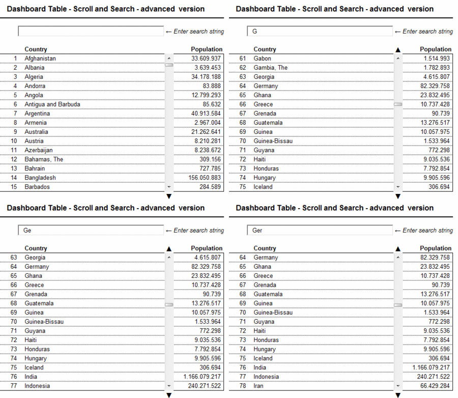
Here is the workbook for free download:

Download Dashboard Table Scroll and Search advanced v01 (Microsoft Excel 2003, 145K)

The Caveat and its Solution

There is one drawback coming with the solutions described above: they are only working properly if the categories (in our example the country names) are sorted alphabetically in the source data. If this is not the case, we have to change the search formula:

=IF(ISNA(MATCH(mySearchString&"*",Data!$C$5:$C$194,0)),1,
MATCH(mySearchString&"*",Data!$C$5:$C$194,0))

The trick is simple: we let the MATCH function look for an exact match by using a zero as the third parameter of the function. Furthermore we concatenate an asterisk to the search string. You probably know the functionality of using wildcards like “*” and “?” in your file searches with Windows Explorer. This functionality is available in Excel’s LOOKUP functions and in the MATCH function as well. If the user types in “Ger”, for instance, the MATCH function looks for “Ger*” and will find the first entry in the database starting with these 3 characters regardless the sort order of the raw data.

Here are the 2 workbooks using this alternative MATCH formula for free download:

Download Dashboard Table Scroll and Search simple v02 (Microsoft Excel 2003, 141.5K)

Download Dashboard Table Scroll and Search advanced v02 (Microsoft Excel 2003, 145K)

What’s next?

At the end of the recent article I announced a follow-up post to Export Microsoft Project Tasks to Outlook. I am still working on that and the article will definitely come during the next few weeks. In the meantime, however, I am planning to write an amendment to Bluffing Tableau Actions with Microsoft Excel, showing a way of how to add better chart tooltips to the World Map visualization.

Stay tuned.

Comments

19 responses to “Scroll and Search in Excel Dashboard Tables”

  1. Chandoo Avatar

    Very cool idea Robert. You dont know how popular your posts are. The KPI posts are still in top 10 visited pages everyday. 🙂

  2. dan l Avatar
    dan l

    I’ve spent the last week with the KPI posts……
    Just saying.

  3. Henrique Avatar
    Henrique

    Excelent! As always!

  4. John Avatar
    John

    Hi Robert ,,,, I use the scroll bar in 3 Excel tables which allow my mgt team to scroll down three separate sets of data for the same set of products ,,, they love it. One question, the raw data I use does have some blank rows ( either hidden or reduced in size ), which the OFFSET function returns a 0 for ,,, and that doesn’t look good in the tables ,,, is it possible to have the formula leave these rows blank and not return a 0 ?

  5. John Avatar
    John

    Hi ,, it’s ok ,, it was as simple as putting in an IFISBLANK statement ,,,, Doh!!

  6. Robert Avatar

    John,
    thanks for your comment.
    Yes, an IF-clause is one option, but you can also use a custom number format like
    “General, General, , General”
    This will hide the zeros as well. However it will hide all zeros, i.e. also the zeros in the raw data.
    Thus, I would recommend the IF-clause with the ISBLANK condition.

  7. Milind Avatar
    Milind

    Hi Robert – Is there a way to protect my sheet, but allowing the user to type in a value in the search box (active x text box).
    I have linked the activex text box to a cell (Y2) that uses the MATCH formula. I have allowed range Y2 to be unprotected. When I try to protect the entire sheet (Y2 is unprotected), and I try to type in the activex text box, I get the message…the cell or chart that you are trying to edit is protected and read only. I dont have a problem if I do not use an activex textbox
    Would appreciate your feedback as always !

  8. Robert Avatar

    Milind,
    thanks for your comment.
    Since I do not know the structure of your workbook, I will refer to the cell ranges of the workbook posted for download in the article (the advanced version):
    The VBA which is called when you enter something in the textbox changes 2 cells on the worksheet control: cell C4 (mySearchPosition) and cell C6 (mySearchString). You have to make sure that both cells are unlocked (Format Cells|Protection|Uncheck Locked).
    I hope this will be helpful.

  9. indra Avatar
    indra

    Hi Robert..Thanks..
    Is there a way to add more data to my sheet?
    I like this tips..

  10. Robert Avatar

    Indra,
    thanks for your comment. No sweat. Only 3 steps necessary:
    1. Go to the data sheet and insert as many rows as you need somewhere within the existing table, e.g. above row 194. This makes sure that all formulas are using the expanded cell range on the worksheet.
    2. Delete the existing data and copy in your own data.
    3. Go to the dashboard and increase the maximum of the scrollbar (right click on the scrollbar and choose properties). In my workbook I have 190 data rows. The dashboard table has 15 rows. Thus, my maximum of the scrollbar is 176. You have to change this according to your number of rows.
    I hope this will be helpful.

  11. Indra Avatar
    Indra

    thx robert..
    it works, but when i change the data with a combination data (number+alphabet) like ; 8Q2DG1S or 53D1F1S, it’s not working.
    i hope you can help me..
    i use this file:
    dashboard_table_scroll_and_search_advanced_v02.

  12. Robert Avatar

    Indra,
    thanks for coming back.
    I checked the file with the examples you provided and it seems to work fine with numericals as well. If you have the 2 examples of your comment as the first 2 entries in your raw data and type in a “5” as the search string, the dashboard table jumps to the second entry. Looks ok from my point of view. Can you please explain what you exactly mean by “it’s not working”?

  13. Damien Avatar
    Damien

    Hi Robert.
    “Option 2 – Use an ActiveX text box to enter the search string” is *almost* exactly what I want…
    I would love it if you could help me tweak it to do the following:
    When using the “search as you type”, I would like it to bring to the top of the list several rows that contain the letters, not just the first one.
    For example, using your data, if I were to type in ‘I’ followed by ‘N’, India, China, and anything else with ‘in’ in it would come up to the top.
    I hope that was clear, I’m a bit of a newbie!

  14. Damien Avatar
    Damien

    And to add to the above, the text needs to be found anywhere within the spreadsheet, not just the first letters of a particular column…

  15. Robert Avatar

    Damien,
    thanks for your comment.
    The workbook is indeed designed to simply search for a string and “jump” to the first entry. It does not change the order of the data, it just automatically scrolls down the table to the first entry that matches the search string.
    What you are asking for would require either sorting or filtering the table according to the string entered. Of course this is possible, but it is out of scope of this article and I can’t answer this in a comment. I hope for your understanding. I will put your idea on my list of possible future blog posts. No promise if or when I will write the article, though.
    Your second request needs some changes in the workbook. If you want to search a string within a matrix (i.e. several columns) instead of an array (one column), one single MATCH formula is not enough. MATCH searches within one column and returns the row of the first occurrence of your search string (or #N/A if not found).
    However, you need 2 results: the row and the column of the first data entry that matches your search string. Thus, you have to do a MATCH on every column of your data. Then you have to find the first column where this MATCH returns a number instead of #N/A. This is the column where your search string is found for the first time and the result of the MATCH formula is the position of the entry in this column.

  16. Meng Avatar
    Meng

    Can I get instructions on how to do that and where, it has been years since I programmed.

  17. Robert Avatar

    Meng,
    there is no need for programming.
    It is just the usual custom number formatting or an Excel formula like =IF(ISBLANK([…],””,[…]).

  18. connie Avatar
    connie

    hi, can anyone help me, I try to follow through both the method, with and without active x but failed. I’m in first time using macros in excel so I’m not sure what went wrong.
    USing the first method for example, I use the cell to enter search string, and as I typed in a letter in the box, it goes into Run-time error ‘1004’: Method ‘Range’ of object ‘_Global’ failed. When I click on “Debug” button, it shows the Sub code of VB Module, yellow highlighted the line ” Range(“myStartPosition”).Value = Range(“myOverwritePosition”).Value”
    When my mouse hover on the line, it says Range(“myStartPosition”).Value =

  19. Robert Avatar

    Connie,
    myStartPosition and myOverwritePosition are named ranges the code is referring to. If the code stops saying “Method Range of Object Global failed”, you probably did not define these names in your workbook or the names in the workbook and the references in the code are different (a typo, maybe).

Leave a Reply

Your email address will not be published. Required fields are marked *