How to create Microsoft Excel dashboards to monitor the progress of a software development project (part 1 of 3)
 When it comes to manage software development projects, you have to monitor a lot of different quantitative and qualitative metrics in order to answer the main question:
“Where are we?”
As in any other project you have to take care of the usual suspects in project controlling like the completion rate of tasks, the milestones and quality gates, the budget adherence, etc. In software development projects, however, there are a couple of very important specific additional facets to be monitored closely:
- The actual status and the trend of software defects
- The test progress, test coverage and test success
- The actual status and the development of change requests
Today’s article is the first of a 3 post series on how to create minimalist, dynamic software project dashboards with Microsoft Excel; this time a software defect monitor dashboard including the Microsoft Excel workbook for free download.
The Challenge
Create a one-page dashboard for monitoring the actual status of software defects in order to have an overview of the software quality at a glance. A dashboard that can be used in your overall project reporting as well.
The Key Performance Indicators
The main metric we care about in this part of the series is the number of software defects. According to Wikipedia a software defect (aka software bug) is
“… the common term used to describe an error, flaw, mistake, failure, or fault in a computer program or system that produces an incorrect or unexpected result, or causes it to behave in unintended ways.”
Usually software defects are categorized by severity, e.g. assigning a defect to one of the following classes:
- Severity 1: Critical
Critical defects result in a total failure of the software or unrecoverable data loss. A workaround is impossible. - Severity 2: Major
Major defects result in massively impaired functionality. A workaround does not exist or is impracticable. - Severity 3: Minor
Minor defects result in non-critical failures of the system. A satisfactory workaround exists. - Severity 4: Cosmetical
Cosmetical defects are of low or very low impairment. A reasonable workaround exists.
Different strokes for different folks. Other projects and other companies may use different naming conventions (like showstopper / severe / medium / minor, or others), but usually there are 4 or maximum 5 categories to classify the severity of a software defect.
The actual status of a software bug can be classified into one of the following 3 main categories:
- Assigned
The defect was detected by Quality Assurance or during other tests (like the User Acceptance Test), assigned to and accepted by the software development team. - Resolved
The defect was detected and assigned to the software development. The bug fix has already been delivered, but it was not yet retested by Quality Assurance. - Closed
The defect was detected and assigned, development delivered the bug fix and Quality Assurance already successfully retested the fix.
Again, terminology may differ across different software projects or companies. Furthermore there are a some more possible status like “in discussion”, “in review”, “rejected”, “duplicate”, etc. Though, in order to keep the showcase lean and simple, I am restricting myself to these 3 defect status.
The Visualizations
- Software defects by severity and status for the actual week
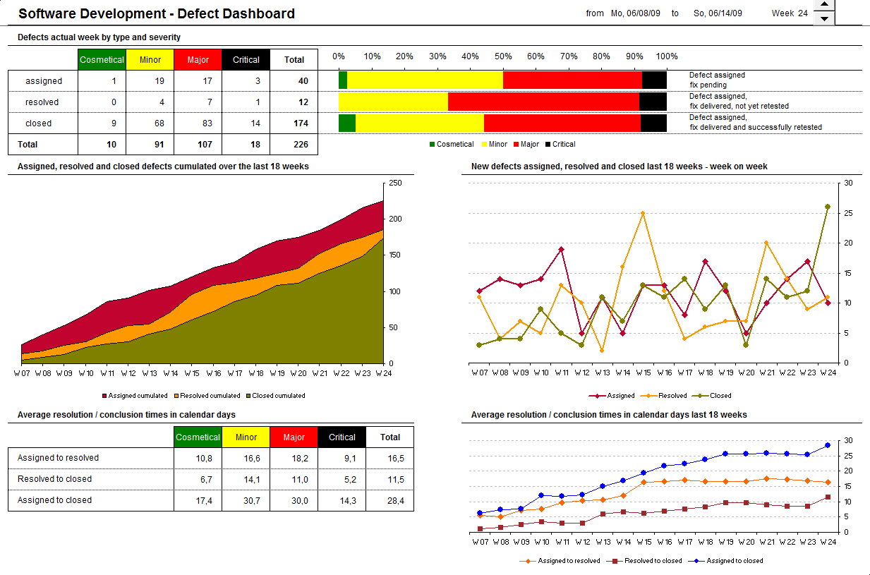
The snapshot of actual number of defects by status and severity is probably the first thing to look at. A simple table enhanced by a stacked bar chart and explanatory texts allows a quick overview:
- Software defects by status over time – cumulated and week on week
An area chart showing the cumulated values of software defects over time and an additional line chart displaying the trend of assigned, resolved and closed defects visualizes all relevant information on the development of software bugs during the project: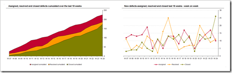 At the beginning of the project we expect the number of assigned defects to grow faster than the number of defects resolved or even closed. Towards the end of the project, however, we should see the cumulated number of assigned defects in the area chart to level off and the gaps between the areas to decrease. With regards to the line chart, this means the orange (resolved) and green (closed) line should tend to be above the red line (assigned) towards the end of the project.
 - Average resolution and conclusion times – actuals and development over time

The average resolution time and average conclusion time are very interesting additional measures regarding the status of software defects. The average number of days between the date of assignment and the date of resolution shows how long software development needs on average to fix a defect. The span between the date of resolution and the date of conclusion reveals the performance of Quality Assurance regarding retesting the delivered fixes. Finally, the period between the date of assignment and the date of conclusion can be used as one of the basic inputs on an estimation to complete.

The visualization is pretty minimalistic: a table displaying the needed average number of calendar days by severity and a line chart showing the evolution of the 3 metrics over time.
The Implementation
As already discussed in a previous post, I am always trying to implement a workbook structure that strictly separates the data input sheet (“data”), the consolidation / calculations (“control”) and the dashboard. This case is no exception.
Hence, you will find all formulas for consolidating the data on the worksheet “control”. There are some advanced formula techniques like array formulas, formulas using SUMPRODUCT and one complex formula calculating the ISO 8601 week numbers. I will not provide a detailed how-to tutorial on these formulas, but the following links might help you understand the used techniques:
- For understanding the concept of array formulas you may want to check out Chip Pearson’s great website
- Charley Kyd has a very good article on his website ExcelUser regarding SUMPRODUCT
- An explanation on how to calculate week numbers is available in a previous post here on Clearly and Simply
Agreed, all these formulas require advanced skills in Microsoft Excel, but they are no rocket science.
The implementation of the used visualizations, however, should be self-explanatory: 2 tables directly linked to the results on the control sheet, a stacked bar chart, an area chart and 2 line charts. Microsoft Excel standard functionality and charts, no tricks and hacks necessary.
The Result
Here is the final result, a screenshot of the complete dashboard:
 A variety of other metrics may be added, like an estimation to complete, the defect fix fault ratio (i.e. the number of bad fixes compared to the number of delivered fixes), etc., but I guess this little showcase should get you going.
The Download Link
Here is the Microsoft Excel workbook for free download:
Download Dashboard Software Development Defect (Excel 97 – 2003, 168K)
All dates and numbers in this workbook are made up.
What’s next?
Monitoring the software defects of your project is only half the battle won. Another extremely important thing to track is the progress and performance of your Quality Assurance and testing. The next article will discuss a Microsoft Excel dashboard to monitor the test progress of a software development project.
Stay tuned.
Comments
33 responses to “Software Project Dashboards – Episode 1”
Minor point: The dark saturated colors of the area chart afford it much greater visual importance than the line charts. A quick calculation in my head tells me that it’s not a stacked area chart. To avoid confusion, this area chart should be changed to a line chart like the one to its right.
Very good as always!
Ill tell you what should be next, to learn some proper dashboard visualization techniques! Plus, the color choices are appalling!
http://www.bonavistasystems.com/OnlineDemoReports.html
Excellent ( as usual ) job.
Great work! Thanks.
Jon,
many thanks for your comment and the constructive criticism. You are right: of course it is not a stacked area chart.
I agree with you: the area chart attracts more attention than the line chart does, but nevertheless I decided to use an area chart for the following reasons:
1. By definition, the cumulated number of assigned defects is always greater or equal than the cumulated number of resolved defects and the cumulated number of resolved defects is always greater or equal than the cumulated number of closed defects. Hence, in this specific case, an area will never hide one of the others.
2. The focus of the chart is on the gaps between the KPIs. We expect and want to watch the gaps to disappear over time, i.e. to see the areas leveling off to a common line. And – from my point of view – this is easier to see with an area chart than with a line chart. Frankly, I am not using area charts very often, but in this specific case I do believe an area chart is the best way to visualize the development of the gaps between assigned, resolved and closed defects.
Let me know what you think.
Some nice ideas on how and what to monitor, but a couple of comments:
Not sure if the %Bar adds anything – the table says it all. What might be of interest is how this week’s defect numbers compare to last week.
Also not sure about the first Line chart – the data’s all over the place making it difficult to decipher and to read anything into the data.
But looking forward to Part 2.
DMurphy,
many thanks for your comment and your suggestions on how to improve the dashboard. Here are my 2 cents:
1. The 100% bar chart
I would agree with you if it would be a standard stacked bar chart. In this case, the chart would indeed add no further information. Using a color-coded 100% bar chart, however, gives a pretty good impression of the distribution of the defects by severity. The more green and yellow you see, the less problems you have and vice versa.
Furthermore you can easily compare the severity distribution of the actual assigned defects to the severity distribution of closed defects (i.e. the average distribution during the whole project so far). Thus, it is pretty easy to see effects like e.g. “this week more than half of all defects are either severe or critical, whereas during the whole project only 30% of all bugs were either severe or critical. Question: Why do we find so many severe and critical bugs that late in time?”
Of course you can derive this information from the table as well, but from my point of view the visualization supports this type of analysis.
2. Compare the actuals to the previous week
I fully agree, comparing the actuals to the last week definitely makes sense. The information is somehow included in the area chart below, but showing last week’s data (at least of the grand totals) in the table as well is a very good idea.
3. The first line chart
I agree, it looks a bit messed and is hard to read and understand. The idea of this chart is less showing the trend but rather comparing the number of assigned, resolved and closed defects week on week. I.e. if the data points of resolved and closed are above the data point of assigned defects, we are doing fine. I thought a line chart would be the best way to visualize the data. But after reading your comment, I fully agree with you. Maybe changing the chart to a dot plot (i.e. a line chart with markers only, but no lines and adding vertical gridlines to seperate the weeks) would help to improve the visualization? What do you think?
Many thanks again for sharing your ideas with us. I greatly appreciate this.
Just perfect!!!as usual..
Thanks for nice info.
I found a rich software testing resources, have a look.
http://SoftwareTestingNet.com
Thanks for the Useful info,
but i have a query, for an assigned defect how will we have a resolved on and closed on date, and i see this data in the datasheet.
Avanish,
many thanks for your comment and question.
I am afraid I do not really understand your question: we have 6 columns on the data sheet: the ID, the severity, the state and the dates for “assigned on”, “resolved on” and “concluded on”. If you detect a new defect, you are supposed to enter the ID, the severity, the state and the date of assignment. As soon as this defect is resolved, you enter the resolution date and – later on – when the defect is closed, you enter the date of conclusion.
Maybe it was a bit confusing that in the example worbook for download all defects already had all date columns filled. During the project, there will be defects that have only dates in the column “assigned on”. As long as a defect is only assigned, the columns for resolved and closed will be empty. At the end of the project however, all defects will hopefully be resolved and closed.
Does this answer your question? If not, can you please elaborate on what exactly your problem or request is? Thanks.
but where I can get a similar dashboard which can be used to monitor sales etc.
Hasan,
have a look at the results of Chandoo’s Visualization Challenge #2 . Chandoo’s readers published a couple of very nice sales dashboards.
This spreadsheet is really fabulous. Great work. How can you set this up so that it handles the turn of the year gracefully? We have defects that date back one (even two years) and we still need to track them. I can’t seem to figure out how to make that work as when the year turns the first week wants to be “known” as WK 01 … and I can’t have two of them in effect at the same time. (this years and last years). Ideas????
Thanks again for providing this.
Steve,
first of all many thanks for your comment and for the appreciation.
The workbook posted for download is indeed limited to 52 weeks. If you need more than one year, you have to change the following:
1. Increase the maximum number of the spin button on the dashboard to the number of weeks you need.
2. The time frame is defined on the worksheet “control” in the cell range B44:D95. Insert the number of additional rows (weeks) somewhere in the middle of this cell range and copy down the formulas from the row above.
3. The start of the time frame is hard coded in cell C44. Set the value of this cell to the Monday of the first week of your project. To make the workbook more general, you could even write a formula there to detect the first date on the data sheet (minimum) and calculate the Monday of the according week, but I think entering a date there once isn’t too much effort.
Actually you can have 2 weeks with the same week number in the spreadsheet, but you will not see the years on the charts’ axes (only the week numbers). However, on top of the dashboard the full dates of the selected week are always displayed.
If you want to see the week number and the year on the axes of the charts, you have to change the formulas in the cell range B19:B36 on the worksheet control. The formula in cell B19 could look like
=TEXT([Existing formula],”W00″)&”/”&TEXT(C19,”YY”)
I hope this will be helpful.
Thank you very much for the advice. I will try this out. Again, thanks for sharing your work here … its quite impressive.
Robert,
I tried all of your changes, but the only issue I have is that I cannot get the spin button to exceed 53 … despite the fact that I extended the date ranges. This kind of makes sense though since the MAX week is 53 due to the fact that when the year turns the first week goes back to WK 01 works its way back up to WK 53 again.
My understanding of the INDEX function is that it will take the first one it hits in the array … which won’t let us page up to the second occurrence of these numbers.
Any suggestions?
Stephen,
you have to increase the maximum value of the spin button. Go to the dashboard, right click on the spin button, choose the tab control and increase the maximum value to the desired number of weeks.
INDEX does not look up a value within the array, but rather navigates to the row defined by the spin button in the cell link.
I hope this will be helpful. If I can be of any further assistance, please let me know.
Never mind. I got it. I had to change the max on the spinner control. I misunderstood your step 1 above … but now I got it. Thanks again. (sorry for all of the replies).
i tried to use this sheet for one of my project however im getting the divide by zero error in Assigned to Resolved
Resolved to Closed and Assigned to Closed fields.
Resolved to Closed(P4): =SUM((Data!$J$2:$J$502=C$40)*(Data!$F$2:$F$504>0)*(Data!$F$2:$F$504<=$C$9)*(Data!$F$2:$F$504-Data!$D$2:$D$504))/SUM((Data!$J$2:$J$504=C$40)*(Data!$F$2:$F$504>0)*(Data!$F$2:$F$504<=$C$9)) Please tell me how to fix it
aman,
those formulas are array formulas.
To enter an array formula, type in the formula and press the CTRL SHIFT and ENTER at the same time, rather than just pressing ENTER. Excel will then automatically enclose the formula in curly braces {}.
If you enter the formula just with ENTER, you will receive the DIV/0 error.
Hi Robert,
This is really useful, I am new to some of the methods you have used in this template.
I was wondering, how best to factor in defects across testing cycles. Any ideas?
Many Thanks
James,
thanks for your comment and question.
It depends on what you mean by “testing cycles”.
If you are talking about different test phases performed one after the other (like system test, global integration test, friendly user test, etc.) you may want to add vertical lines or shaded bands to the area and line charts to visualize the beginning and the end of the different test phases. Or add a bar or stacked bar chart showing the total numbers of defects per test phase.
This is good. I was looking for some handy template for dashboards for quite some time. But I think now my search is over, as I found something which is closer to what I want to prepare. I can certainly build upon these templates. Thanks for sharing.
Awesome job, I was wondering if there is anything that give holistic view on cost estimate and productivity
kwiz,
thanks for your comment. Sure, you may visualize any type of information on a project report dashboard like this. It depends on the data you have available and what exactly you want to visualize.
Actual project cost versus budget could be displayed using e.g. a line chart with 2 data series (if you want to show development over time) or a simple thermometer bar chart or a bullet chart (if you focus on the actual status only).
Productivity could be shown on a burn down chart, for instance.
As mentioned above, it always depends on what you are exactly looking for and what data you have available.
First off I love the spreadsheet. I have been in the process of reverse engineering it so that I understand how it all works. What I do not understand is how the SUMPRODUCT formula works?
For example:
=SUMPRODUCT((D$4=’Data Defects’!$C$5:$C$504)*(‘Data Defects’!$E$5:$E$504>0)*(‘Data Defects’!$E$5:$E$504<='Control General'!$C$10)*(('Data Defects'!$F$5:$F$504=0)+('Data Defects'!$F$5:$F$504 >‘Control General’!$C$10))*((‘Data Defects’!$G$5:$G$504=0)+(‘Data Defects’!$G$5:$G$504>’Control General’!$C$10)))
Is it possible for you to explain how this formula works and break it down?
Thanks
Savvy,
it seems as if the formula you posted is from your reengineered workbook (with apparently a sheet Data Defects and one called Control General), so I am not 100% sure which formula you are referring to, but I assume it may be the one used in the crosstab of status and severity, right?
To make it easier for me and the other readers, I will refer to the original workbook posted above. In the original workbook, the formula in cell C13 of the Control worksheet calculates the number of cosmetical defects with status “assigned”:
=SUMPRODUCT(
(C$12=Data!$C$5:$C$504)*
(Data!$E$5:$E$504>0)*
(Data!$E$5:$E$504<=$C$9)* ((Data!$F$5:$F$504=0)+(Data!$F$5:$F$504>$C$9))*
((Data!$G$5:$G$504=0)+(Data!$G$5:$G$504>$C$9)))
I will try to break it down by using pseudo code:
(severity = “Cosmetical”) AND
(date assigned on > 0) AND
(date assigned on <= Sunday of selected week) AND ((date resolved on = 0) OR (date resolved on > Sunday of selected week)) AND
((date closed on = 0) OR (date closed on > Sunday of selected week))
Each line creates a Boolean array (TRUE if meeting the condition, FALSE if not) and the SUMPRODUCT counts all data records meeting all conditions. Instead of SUMPRODUCT you could also use SUM and enter the formula as a matrix formula (CTRL-SHIFT-ENTER).
I hope this will be helpful.
Hi Robert, hi folks!
First, thank you for the Dashboard. I’m having many issues with this. I have adapted your dashboard to my projetc and when I’d like to understand why status “Assigned to resolved”, “Resolved to closed” and Assigned to closed” are displaying a huge number, like 41.555,00. I know its happening because i didn’t put any date, but how to not display this number, or how not count it?
Even why if my project is running, some status are not fully filled…and it’s incorrect! Calculate something when it’s not happen…
Felipe,
as you said, large numbers in the resolution / conclusion times will occur if you have a date for “resolved on” and / or “concluded on” but no date for “assigned on”. In this case, the missing “assigned on” date will be treated as zero, i.e. December 31st, 1899. This will result in a resolution time of more than 41,000 days (days since 12/31/1899).
The concept and design of this dashboard heavily rely on dates (and weeks). Hence, the dates are mandatory. Not only for the calculation of resolution and conclusion times, but also for all other tables and charts like the area and line chart in the middle of the dashboard. In other words: if you do not have an assignment date of a defect, it doesn’t make sense to have it in the data at all, because it will not be displayed in any of the tables and charts.
Thank you Robert! I really understand your point.
But, incase I want to exclude to count this cells, that contain ZERO, cos Im adapting…
I’ve tried this
=SUM((Data!$I$5:$I$504>0)*(Data!$I$5:$I$504<=$D19)*(Data!$I$5:$I$504-Data!$H$5:$H$504=12/31/1899))/SUM((Data!$I$5:$I$504<=$D19)*(Data!$I$5:$I$504>0))
Or, how you would do it??
Felipe,
if you want to exclude records without assignment date from the calculation of resolution and conclusion times, you have to add a Boolean vector to all array formulas to ensure only records with assignment dates greater than zero will be included in the sum.
For instance, the formula in E39 (“Assigned to resolved” / “Major”) would be the following (array-entered):
=SUM(
(Data!$C$5:$C$504=E$38)*
(Data!$E$5:$E$504>0)*
(Data!$F$5:$F$504>0)*
(Data!$F$5:$F$504<=$C$9)* (Data!$F$5:$F$504-Data!$E$5:$E$504))/ SUM((Data!$C$5:$C$504=E$38)* (Data!$E$5:$E$504>0)*
(Data!$F$5:$F$504>0)*
(Data!$F$5:$F$504<=$C$9)) The 2 parts "(Data!$E$5:$E$504>0)” are the Boolean vector I mentioned above.
You have to change all formulas accordingly in the ranges N19:P36 and C39:G41.